[Paper Review, EN] MotionStream: Real-Time Video Generation with Interactive Motion Controls

Paper Information
Title: MotionStream: Real-Time Video Generation with Interactive Motion Controls
Authors: Joonghyuk Shin, Zhengqi Li, Richard Zhang, Jun-Yan Zhu, Jaesik Park, Eli Shechtman, Xun Huang
Venue: ICLR 2026 Oral
Link: [Paper], [Project], [GitHub]

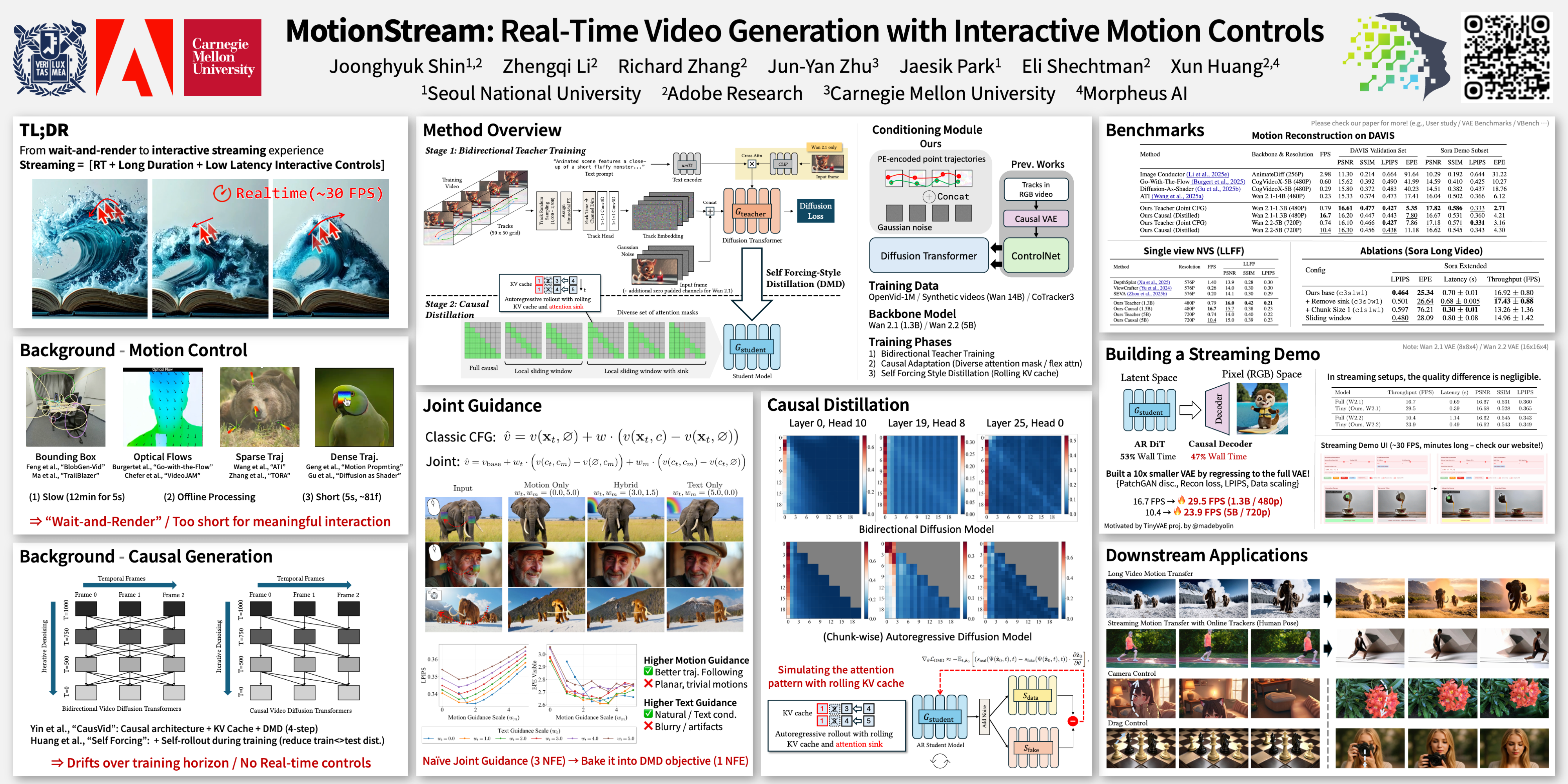
Teaser Image (Poster)

Introduction

Motion-controlled video generation has evolved to allow users to directly specify the motion of objects, people, and cameras. Early controllable video generation research explored various conditions such as structure, camera, subject, and audio, and as motion itself became an important conditioning signal that directly represents video dynamics, diverse motion representations such as optical flow, 2D/3D trajectories, bounding boxes, and semantic segmentation began to be used. Recent video diffusion models have achieved high visual quality and precise trajectory following using these conditions, but most are based on bidirectional diffusion architectures that process the entire video and the full motion condition at once. Therefore, users must specify the complete future trajectory in advance, and it is difficult to inspect intermediate results or modify motion during generation. In addition, the iterative denoising process of diffusion makes generation very slow; the paper cites Motion Prompting as an example, which takes about 12 minutes to generate a 5-second video. Ultimately, despite their high quality and controllability, existing motion-controlled video generation methods are not suitable for real-time interaction because of slow generation speed, non-causal processing, and short generation lengths.

Meanwhile, temporal generation in video generation began with early GAN-based autoregressive/parallel video synthesis and later evolved into video diffusion models trained with denoising objectives and autoregressive video models based on next-token prediction. More recently, active research has combined the two paradigms to build causal yet high-quality AR-diffusion models. In particular, distilling a slow bidirectional diffusion teacher into a fast autoregressive student has increased the possibility of real-time generation, but these models can accumulate color drift or quality degradation when generating far beyond the sequence length seen during training, or require complex long-video fine-tuning to prevent such issues. At the same time, interactive video world models such as the Genie family have also advanced toward real-time user interaction, but many methods require substantial inference compute or are limited to closed-domain or synthetic environments such as Minecraft and games. Thus, prior work has achieved subsets of controllability, causal generation, and real-time interaction, but stable, long-horizon real-time generation with motion control in open-domain photorealistic video remains an unresolved challenge.

Method & Technical Details

Adding Motion Controls to Bidirectional Teacher Models

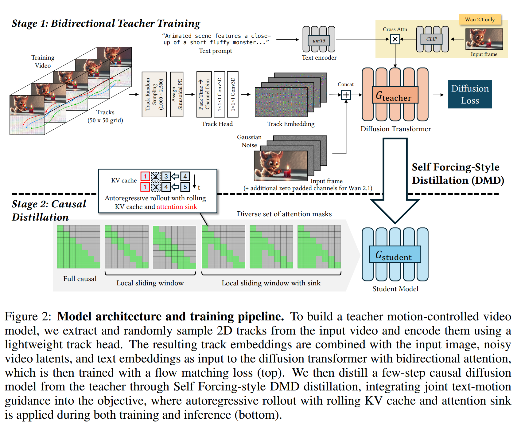
The key idea of this technique is:

to build a teacher model by adding motion-trajectory conditioning capability to an existing Wan-family bidirectional video diffusion model

This is the core idea.

In other words, this stage builds a high-quality teacher that follows motion accurately.

First, we need to consider how to represent the input motion. In other words, let us look at Track Representation.

The input motion is represented as multiple 2D point trajectories. Suppose a point $n$ moves over time as

\[(x_t^n, y_t^n)\]

We can think of it as moving in this way. Each track is assigned a unique $d$-dimensional embedding $\phi_n$. This embedding is not a learnable ID embedding; instead, it is obtained by applying sinusoidal positional encoding to a random ID. That is,

• track 1 $\rightarrow$ $\phi_1$
• track 2 $\rightarrow$ $\phi_2$
• track 3 $\rightarrow$ $\phi_3$

This gives each trajectory an identity that distinguishes it from the others. At each frame $t$, the corresponding embedding is placed at the track location. (This may look complicated because several technical terms appear at once. Open the detail section below for a more detailed explanation.)

Track Representation

The concept of a track appears frequently in many 4D Generation papers. A track can be understood as a representation that tells us where a point moves as the video frame changes.

For example, if a point is at $(100,200)$ when $t=1$ and moves to $(105,201)$ when $t=2$, we can represent this track as follows:

\[\{(x_t^n, y_t^n)\}_{t=1}^T = \{(100,200), (105,201)\}\]

MotionStream tracks points in the actual training data using a model called CoTracker3. It tracks 2,500 points with CoTracker3 and randomly samples 1,000–2,500 of them during training.

The paper states that each 2D track is assigned a randomly sampled ID number. However, rather than feeding a scalar ID number directly into the model, it is useful to convert it into a high-dimensional vector, so the ID number is transformed into a $d$-dimensional vector. This is called an embedding. MotionStream sets $d=64$, representing the ID of each track as a 64-dimensional vector.

For example,

\[ID = 17\]

for a track with this ID, the ID is converted into

\[\phi_{17} = [0.21, -0.84, 0.56, ...] \in \mathbb{R}^{64}\]

The ID is transformed in this way. The method used to convert the ID into a vector is Sinusoidal Positional Encoding. For an ID $p$,

\[[sin(p),cos(p),sin(p/10),cos(p/10), ...]\]

it creates a single vector from sin/cos values at multiple frequencies. The key point is that different IDs produce different vectors.

The following equation then appears.

\[c_m \left[ t, \left\lfloor \frac{y_t^n}{s} \right\rfloor, \left\lfloor \frac{x_t^n}{s} \right\rfloor \right] = v[t, n]\phi_n\]

This equation means placing the embedding at a location downsampled to match the VAE latent resolution.

First, $c_m$ is the motion-conditioning tensor. The paper defines its shape as $c_m \in \mathbb{R}^{T \times H/s \times W/s \times d}$. The axes correspond to (time, vertical position, horizontal position, track embedding). In other words, each frame has an $H/s \times W/s$ map, and each location can store a $d$-dimensional vector.

The original track locations are coordinates in the original video pixels. For example, suppose the spatial compression factor is $s=8$ and $H=480, W=832$. Because the diffusion model processes VAE-compressed latents rather than the original RGB video directly, $480 \times 832$ is reduced to approximately $60 \times 104$. Therefore, if a track in the original pixels is at

\[(x,y) = (320,160)\]

then in latent coordinates it becomes

\[(\frac{320}{8}, \frac{160}{8}) = (40,20)\]

Thus, the equation uses

\[\left\lfloor \frac{y_t^n}{s} \right\rfloor, \left\lfloor \frac{x_t^n}{s} \right\rfloor\]

For track visibility, not every track is visible in every frame. For example, if a person is occluded behind another person, a particular point may not be visible. This is represented by

\[v[t,n] \in \{0,1\}\]

When it is visible, the value is 1, so

\[c_m[ \cdots ] = \phi_n\]

and when it is occluded and not visible, the value is 0, so

\[c_m[ \cdots ] = 0\]

Thus, $v[t,n]$ acts as a visibility mask. Next, let us look at the Track Head. Instead of feeding the constructed $c_m$ directly into the diffusion transformer, it is first passed through a small network called the track head.

The overall flow is roughly

\[\text{2D Tracks} \rightarrow \text{Sinusoidal ID Embedding} \rightarrow c_m \rightarrow \text{Track Head}\]

The Track Head first performs 4x temporal compression. This is because Wan’s VAE also compresses the video latent along the temporal axis. The original tracks exist at every frame, but the video latent has a lower temporal resolution, so the motion condition must be matched to the same temporal resolution.

It then applies a $1 \times 1 \times 1 \;\; Conv3D$. This convolution is a lightweight layer that projects the feature vector at each location to the desired channel dimension.

Existing controllable diffusion methods often use a ControlNet-style architecture, but this paper adopts a simpler design. The authors explain that ControlNet adds another network branch similar to the backbone, substantially increasing computation. Therefore, it is not used because it conflicts with MotionStream’s goal of real-time rendering.

The motion feature processed by the track head is therefore concatenated directly with the video latent along the channel dimension:

\[[\text{video latent} || \text{motion feature}]\]

This adds motion control without duplicating the backbone as in ControlNet.

Next, we discuss how this teacher is trained. The authors train it with a rectified flow matching objective. Conceptually, the input is $z_t + \text{text} + \text{motion condition}$, and the output is a $\text{velocity prediction}$. Thus, the teacher is trained as a video generator that follows both the text and the track trajectory.

However, there is a problem. In the previous equation, $v[t,n]$ was used to represent track visibility. When this value is 0, the motion feature at that location also becomes 0. If the user stops providing control during interaction, the motion signal disappears, which also produces a value of 0. From the model’s perspective, it is therefore difficult to distinguish whether a zero means that a track is occluded or that the user has stopped specifying the track.

This can cause the model to interpret a disappearing track as a disappearing object. The paper explains that this can produce artifacts in which objects suddenly appear or disappear. To address this, the paper uses Stochastic mid-frame masking.

This method intentionally removes the motion signal from some frames. In the paper,

\[c_m[t_{rand}, :, :] = 0\]

and the probability is set to $p_{mask}=0.2$. The purpose is to train the model so that the video remains coherent even when the motion condition suddenly disappears in the middle. This strategy is not used from the beginning; the model is first trained without it to learn accurate motion-track following, and the masking is introduced afterward.

The paper denotes the text condition by $c_t$ and the motion condition by $c_m$, and the two conditions play different roles. However, if one guidance term becomes too strong, the object may move in an overly rigid and simplistic manner (when motion guidance is too strong), or it may deviate from the user-specified trajectory (when text guidance is too strong).

Therefore, the two guidance terms must be balanced, and the authors use joint guidance:

\[\hat{v} = v_{\mathrm{base}} + w_t \left( v(c_t, c_m) - v(\emptyset, c_m) \right) + w_m \left( v(c_t, c_m) - v(c_t, \emptyset) \right)\] \[v_{\mathrm{base}} = \alpha v(\emptyset, c_m) + (1-\alpha)v(c_t, \emptyset), \qquad \alpha = \frac{w_t}{w_t+w_m}\]

Because the MotionStream teacher is a rectified flow model, at each denoising step it observes the current noisy latent $z_t$ and predicts the velocity $v(z_t, t, c_t, c_m)$. It then follows this velocity to move the latent gradually toward a clean video. Instead of simply using $v(c_t, c_m)$, however, the model constructs a final velocity that emphasizes the influence of the text and motion conditions, similar to CFG. This is exactly what the equation for $\hat{v}$ above describes. The flow is therefore

\[\text{Model Predictions} \rightarrow \text{joint-guided } \hat{v} \rightarrow \text{next denoising step}\]

The equation for $\hat{v}$ is more complicated than simply using $v(c_t, c_m)$. It is based on the idea of CFG: measure how much the prediction changes when a condition is present versus absent, and amplify that difference.

Here,

\[v(c_t, c_m) - v(\cancel{0}, c_m)\]

represents the text effect, indicating the direction added to the velocity prediction by the text. Multiplying by $w_t$ controls the strength of the text influence. Conversely,

\[v(c_t, c_m) - v(c_t, \cancel{0})\]

keeps the text the same and changes only the motion. Therefore, it can be viewed as the direction added by the motion trajectory, and multiplying by $w_m$ controls motion adherence. The $v_{base}$ equation below $\hat{v}$ also mixes motion-only and text-only predictions.

This joint guidance also has a drawback. Although it improves quality, it increases computation because each denoising step must evaluate

\[v(c_t, c_m), v(\cancel{0}, c_m), v(c_t, \cancel{0})\]

separately, requiring 3 NFE (Number of Function Evaluations). Therefore, the teacher itself is not a real-time model.

In summary, the most important techniques used to train the teacher model are Track Representation, Track Head, Stochastic Mid-frame Masking, and Joint Text-Motion Guidance.

Causal Distillation

The teacher model is currently a bidirectional diffusion model. For example, when generating an 81-frame video, the teacher attends to all frames simultaneously. Thus, even when processing a particular 10-frame portion, it can use the entire 1–81 temporal context. This is advantageous for producing high quality, but problematic for real-time interaction. If the user has not yet drawn a future trajectory, there is no control signal for those future frames. Therefore, this setup is unsuitable for a real-time setting in which the model must immediately generate video using only the trajectory provided so far. Thus,

the student must become a causal model that generates the next part using only previously generated outputs, following $1 \rightarrow 2 \rightarrow 3 \rightarrow …$.

The paper explains that directly using the Self Forcing approach with causal attention also causes problems. The first is that quality collapses rapidly outside the training horizon. If the teacher was trained on videos of about 81 frames, the student may generate videos of a similar length well, but once generation extends beyond that horizon, errors can accumulate and geometry can become unstable.

The second issue is that latency is not constant when the attention context grows with sequence length. With full causal attention, the past keeps accumulating as the number of frames grows, so the context also becomes larger. As a result, attention cost increases for longer videos, which is critical for real-time streaming.

Therefore, MotionStream uses Sliding Window Attention, a simple approach that attends only to a recent subset of the past rather than the full history. However, this also creates a problem. During long generation, if information from the first input image falls outside the window, small errors can accumulate from frame to frame. This is referred to as autoregressive error accumulation / drift.

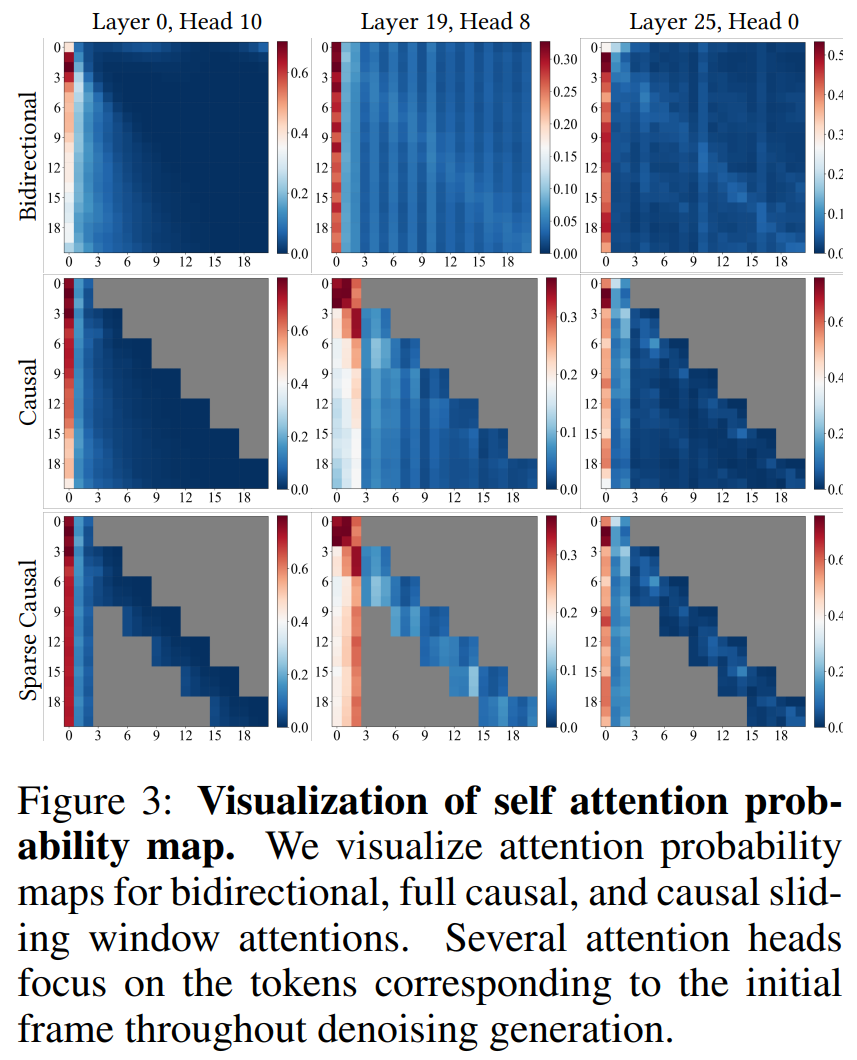
The authors then directly inspect the self-attention maps shown in Figure 3 above. They observe that, in both bidirectional and causal settings, many attention heads continue to attend strongly to the tokens of the initial frame. From the model’s perspective, the first frame is not merely an old frame; it serves as an “anchor for preserving the video’s identity and scene”. The authors view this as analogous to the attention sink phenomenon identified in StreamingLLM.

Therefore, the authors propose the following:

use a sliding window while never discarding the very first frame.

Because the first chunk remains fixed, the paper explains that it can continue to anchor the original scene and identity even during long generation. This is called the sink chunk.

Now we need to understand the rolling window used in the paper. We have already discussed why the sink and the window are needed and what they are. This gives us two hyperparameters:

\[S = \text{number of sink chunks}, W = \text{local window size}\]

If $S=1, W=2$ and chunk 11 is being generated, the context is $[1,9,10]$. In other words, the sink chunk stays fixed while only the local window moves.

We now understand how the student operates. However, directly transferring the bidirectional teacher weights to the causal student does not work well. The teacher was originally trained to see both the past and the future, whereas the student can only see the past. Therefore, the student is first initialized from the teacher weights and then adapted to the causal architecture. For this, attention masks with different context window sizes and attention sink sizes are used. This prevents the student from overfitting to a single causal pattern and helps it adapt to diverse causal contexts. The authors call this Causal Adaptation.

Now we can describe the distillation method in detail. MotionStream adopts a distillation method based on the existing Self-Forcing approach. In standard autoregressive training, a ground-truth previous frame is typically provided as the condition, and the model predicts the next frame. The problem is that ground truth is unavailable at inference time.

Therefore, the model must reuse its own generated outputs as conditions. During training it sees clean inputs (GT), whereas during inference it must repeatedly consume inputs containing its own errors. This is the train-test gap. Self Forcing addresses this by making the model use its own generated outputs as the next inputs during training, just as it does at inference time.

Now let us describe how MotionStream distillation works.

First, the paper divides the entire video latent into $L$ chunks.

\[\{z_t^i\}_{i=1}^L\]

Here, $i$ is the chunk index. The paper defines the context used to generate the current $i$-th chunk as

\[C_i = \{z_t^i\} \cup \{z_0^j\}_{j \le S} \cup \{z_0^j\}_{\text{max(1, i-W)} \le j < i}\]

This can be interpreted as “current noisy chunk + initial sink + recent generated chunks”. Therefore, the probability of the entire video is

\[p_{\theta}(z_0^{1:L}) = \prod_{i=1}^{L} p_{\theta}(z_0^i \mid C_i)\]

This means generating chunk 1, then generating chunk 2 conditioned on it, then chunk 3 conditioned on the previous outputs, and so on. In other words, this is causal autoregressive generation.

In addition, MotionStream uses a concept called Rolling KV Cache. If all past KV states are stored, memory and attention cost continue to grow, so MotionStream retains only Sink KV + Recent window KV. The portion of the KV cache that is continuously updated is therefore the window chunks rather than the sink chunk. For example, if $S=1, W=2$, when generating chunk 10 the cache contains [1,8,9], and after chunk 10 is generated the KV cache is updated to [1,9,10].

Training also uses this rolling behavior. Some prior methods use a causal attention mask during training but apply a rolling cache only at inference, creating a mismatch between training and inference. MotionStream therefore uses

\[\text{self-rollout} + \text{rolling KV cache} + \text{attention sink}\]

during training as well, and the paper refers to this as extrapolation-aware training. The distillation method adopts the existing DMD approach. For a detailed explanation of DMD, refer to the Preliminary section of the FlashWorld paper-review post.

DMD is used for distillation, but the teacher uses both text guidance and motion guidance. As a result, teacher inference requires 3 NFE, which would undermine the real-time generation goal if retained by the student. Therefore, this expensive guidance is distilled into the student so that it is built in. In DMD, the teacher is used as $s_{real}$, i.e., as the score estimator.

\[s_{\mathrm{real}} = s_{\mathrm{base}} + w_t \left( f_\phi(c_t,c_m)-f_\phi(\emptyset,c_m) \right) + w_m \left( f_\phi(c_t,c_m)-f_\phi(c_t,\emptyset) \right)\]

This is almost identical to the equation previously used to compute the teacher model’s final guided velocity $\hat{v}$. The paper describes it as the equation for constructing the real-data score. In contrast, the fake score estimator is

\[s_{fake} = f_{\psi}(c_t, c_m)\]

which uses only a single evaluation without CFG. Thus, at inference time the student does not need to separately compute text CFG and motion CFG. This is what it means to distill the expensive guidance into the student.

Two networks appear here: the student Generator $G_{\theta}$ that actually generates the video, and the fake score estimator $f_{\psi}$ that estimates the score of the distribution currently produced by the student.

\[\nabla_{\theta} L_{\mathrm{DMD}} \approx - \mathbb{E}_{t,\hat{z}_0} \left[ \left( s_{\mathrm{real}}(\Psi(\hat{z}_0,t),t) - s_{\mathrm{fake}}(\Psi(\hat{z}_0,t),t) \right) \cdot \frac{\partial \hat{z}_0}{\partial \theta} \right]\]

Looking at the DMD equation, we can see that the goal is to train the Generator for real-time generation. In other words, the objective is to update the Generator parameters $\theta$ using the difference between the score $s_{fake}$ estimated by the critic and the teacher score $s_{real}$.

The paper uses a 1:5 update ratio between the generator and critic, training the critic more frequently so that it can closely track the current generator distribution.

The method also uses Gradient truncation. Storing gradients for the entire autoregressive self-rollout requires substantial memory because the computation graphs for multiple denoising steps across all $L$ chunks would otherwise need to be retained. Therefore, MotionStream applies the gradient truncation strategy used in Self-Forcing.

One denoising step is randomly selected, and gradients are backpropagated only through that step. In addition, the KV cache from previous frames is treated as stop-gradient, preventing gradients from propagating back through the past cache. This greatly reduces memory usage.

Inference

After training the Student Generator with DMD, inference keeps only

\[\text{sink chunks} + \text{recent local chunks}\]

in the KV Cache. Each time a new chunk is generated, the local window rolls forward by one position. As a result, the attention context size does not increase no matter how long the video becomes. Therefore, the per-chunk computational cost remains approximately constant as video length grows.

Experiments

Implementation details

MotionStream uses Wan 2.1 I2V 1.3B and Wan 2.2 I2V 5B as backbones. The teacher model is trained using OpenVid-1M and synthetic videos generated by Wan T2V models, with approximately 70K synthetic samples for Wan 2.1 and 30K for Wan 2.2. During causal adaptation and Self Forcing distillation, input images, text prompts, and 2D motion tracks are sampled from these synthetic datasets. Motion tracks for all real and synthetic videos are extracted from a 50×50 uniform grid using CoTracker3, and detailed training settings are provided in the Appendix.

Quantitative Evaluations

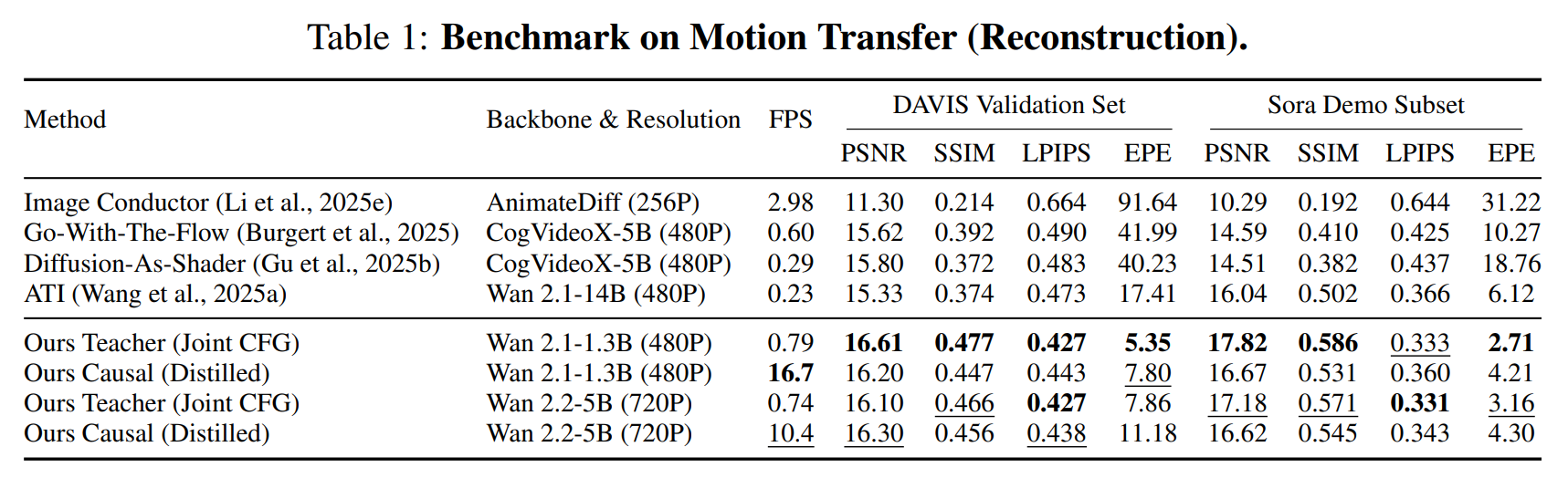
The quantitative evaluation covers two tasks: Motion Transfer and Camera Control. For Motion Transfer, the authors use 30 videos from the DAVIS validation set and 20 videos from a curated Sora demo subset, directly comparing generated results with the corresponding ground truth. Visual fidelity is measured with PSNR, SSIM, and LPIPS, while motion-following accuracy is measured by EPE (End-Point Error) between the input tracks and tracks extracted from the generated videos. In Table 1, MotionStream’s teacher and causal student show strong reconstruction and motion-following performance compared with existing motion-controlled video generation methods. Although the causal student exhibits some quality degradation relative to the teacher, it achieves high generation throughput of 16.7 FPS at 480P and 10.4 FPS at 720P.

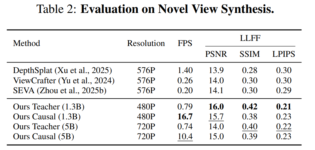
For Camera Control, MotionStream applies its 2D track control zero-shot to single-image novel view synthesis and evaluates it on the LLFF dataset. It first estimates the geometry of the input image using monocular depth estimation, then uses the depth and camera parameters to derive 2D motion trajectories from the input view to the target view, which serve as the motion condition. In Table 2, compared with DepthSplat, ViewCrafter, and SEVA, MotionStream achieves strong PSNR, SSIM, and LPIPS performance despite not being a dedicated 3D novel-view synthesis model. In particular, the causal model maintains substantially higher throughput than both the existing baselines and the bidirectional teacher.

Ablation Experiments

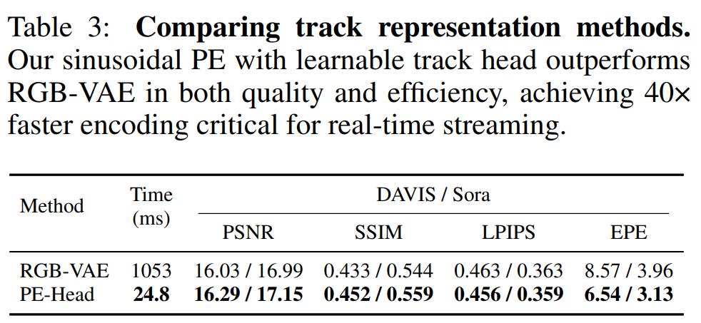
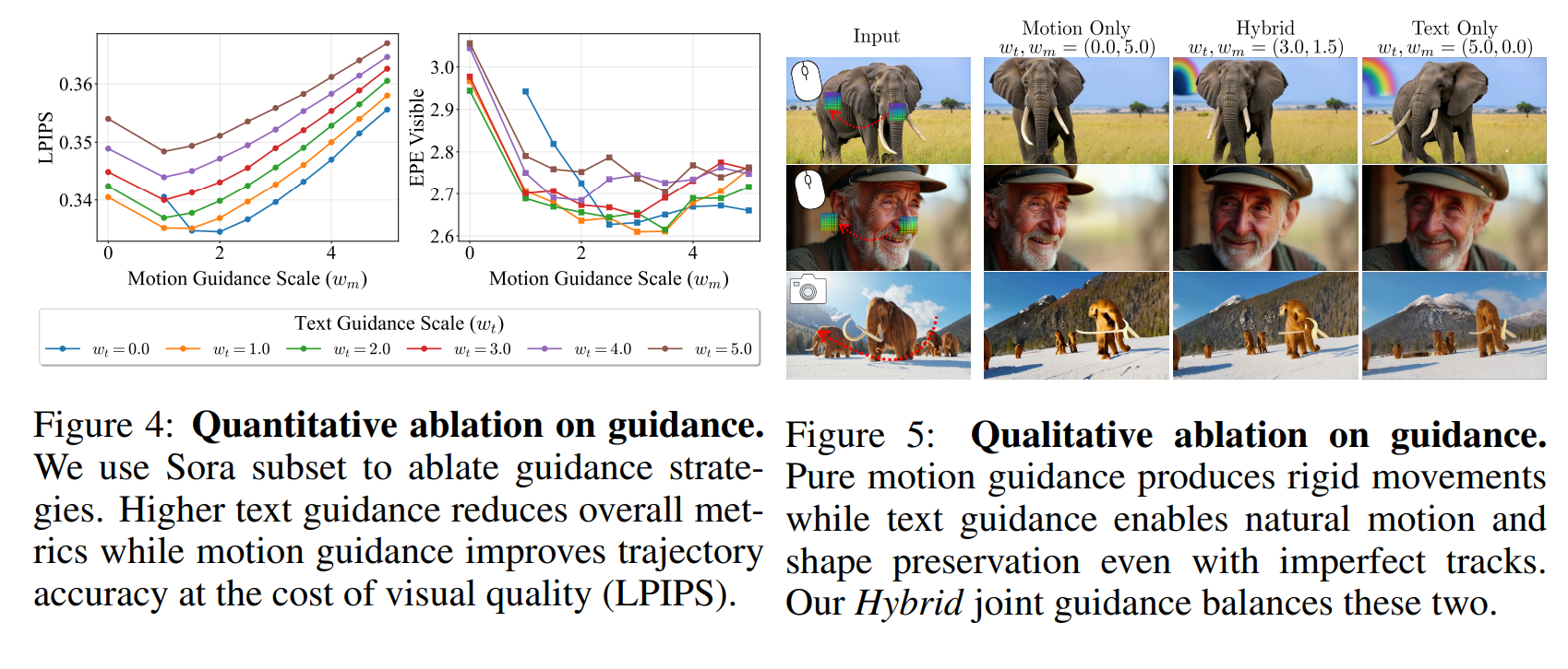
The ablation study analyzes three main components: track representation, text-motion guidance, and the chunk/sink/window design. Table 3 compares the conventional RGB-VAE-based trajectory encoding with the proposed sinusoidal positional encoding + learnable track head. Because the proposed method does not pass the tracks through a VAE, encoding time is greatly reduced while motion alignment and video quality are improved, making it better suited for real-time streaming. Figures 4 and 5 then analyze the balance between text guidance and motion guidance. Stronger motion guidance improves trajectory adherence but can make motion rigid and reduce visual quality, whereas text guidance produces more natural and diverse dynamics at the cost of trajectory accuracy. The paper therefore uses joint guidance with $w_t=3.0, w_m=1.5$ to balance these properties.

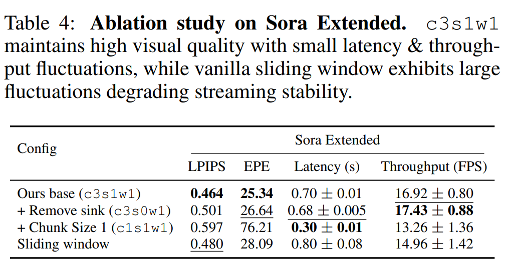
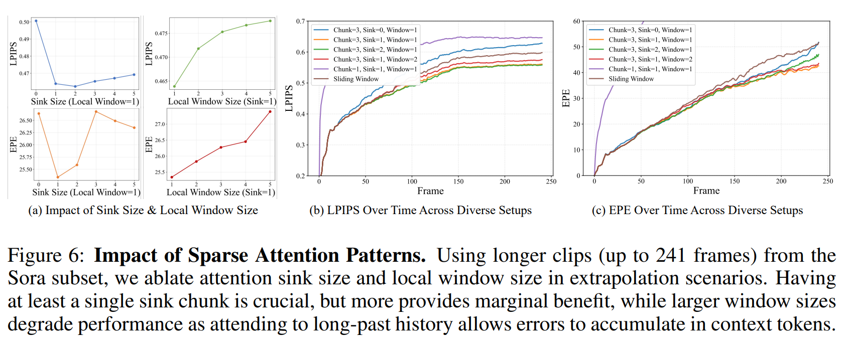
The paper also analyzes chunk size, attention sink size, and local window size for long-video streaming. Table 4 and Figure 6 show a trade-off: if the chunk size is too small, more autoregressive rollouts are required, reducing quality and throughput; if it is too large, latency increases. The final choice is a chunk size of 3. A single attention sink already makes a substantial contribution to suppressing long-term drift, while adding more sinks provides little additional benefit. In contrast, enlarging the local window causes the model to attend to older self-generated context, increasing error accumulation and degrading performance. The final configuration is therefore c3s1w1 (chunk 3, sink 1, window 1), which maintains stable quality in long videos with small latency and throughput fluctuations.

Streaming Demo and Qualitative Results

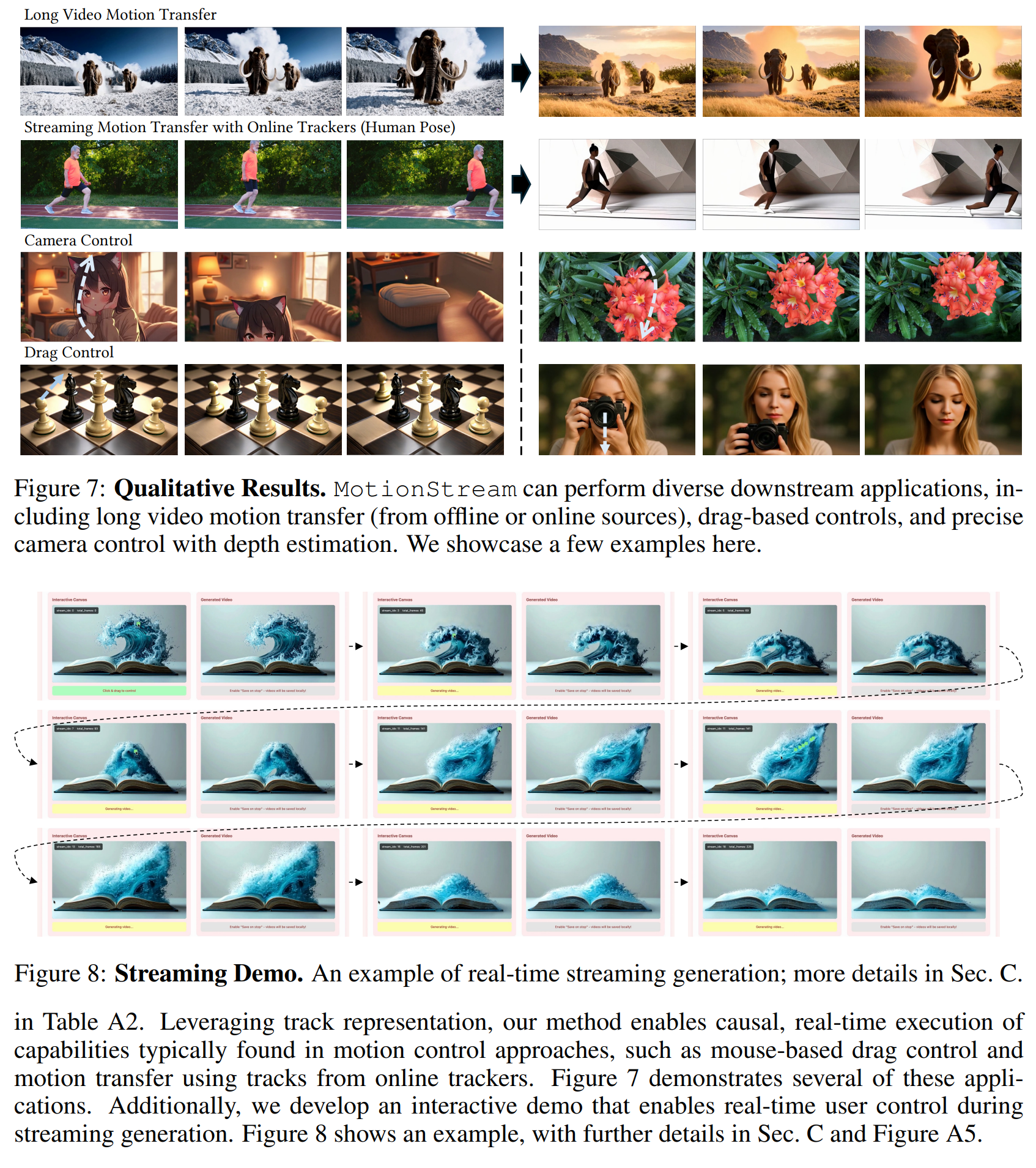
For real-time streaming, the authors additionally train a Tiny VAE decoder to reduce the VAE decoding bottleneck. This accelerates the Wan 2.1-based model from 16.7 FPS / 0.69s latency to 29.5 FPS / 0.39s latency, and the Wan 2.2-based model from 10.4 FPS / 1.1s to 23.9 FPS / 0.49s. Figure 7 presents diverse applications including long-video motion transfer, drag-based control, and camera control, while Figure 8 presents an interactive streaming demo in which users can manipulate trajectories in real time during generation.

Limitations & Future Work

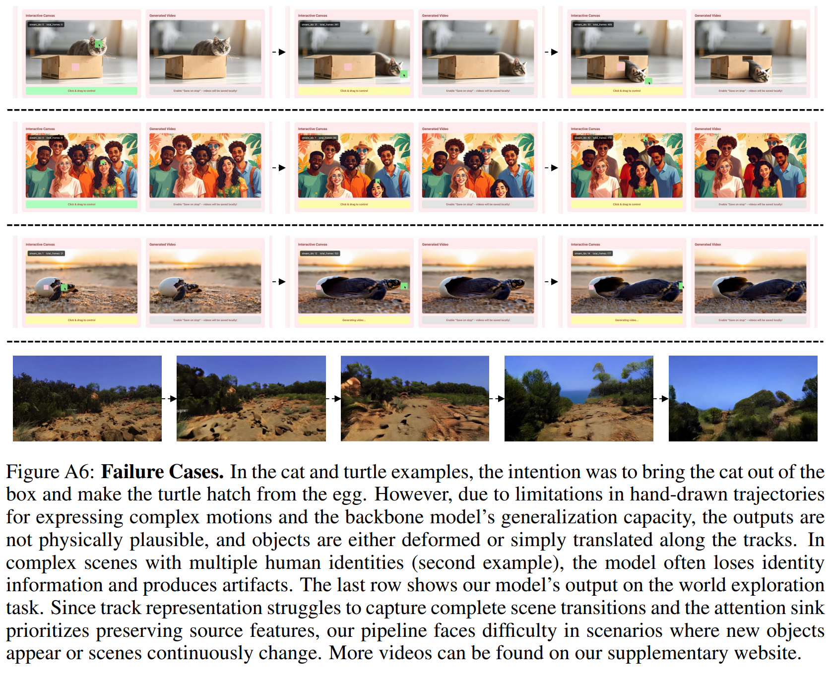
• Because the fixed attention sink strongly anchors the model to the initial scene, it is unsuitable for long-term world exploration involving complete scene changes. The paper therefore proposes dynamic attention sink / anchor refresh as future work.
• Extremely fast or physically implausible trajectories can cause temporal inconsistencies or object deformation, motivating more diverse track augmentation and the use of larger backbones.
• In complex scenes or with complex text and motion, preserving source details and identity can be difficult, which is related to limitations in backbone capacity and image-conditioning mechanisms.