[Paper Review, KR] Diff4Splat: Repurposing Video Diffusion Models for Dynamic Scene Generation

Paper Information
Title: Diff4Splat: Repurposing Video Diffusion Models for Dynamic Scene Generation
Authors: Panwang Pan, Chenguo Lin, Jingjing Zhao, Chenxin Li, Yuchen Lin, Haopeng Li, Honglei Yan, Kairun Wen, Yunlong Lin, Yixuan Yuan, Yadong Mu
Venue: CVPR 2026
Link: [Paper], [Project], [GitHub]

Teaser Image

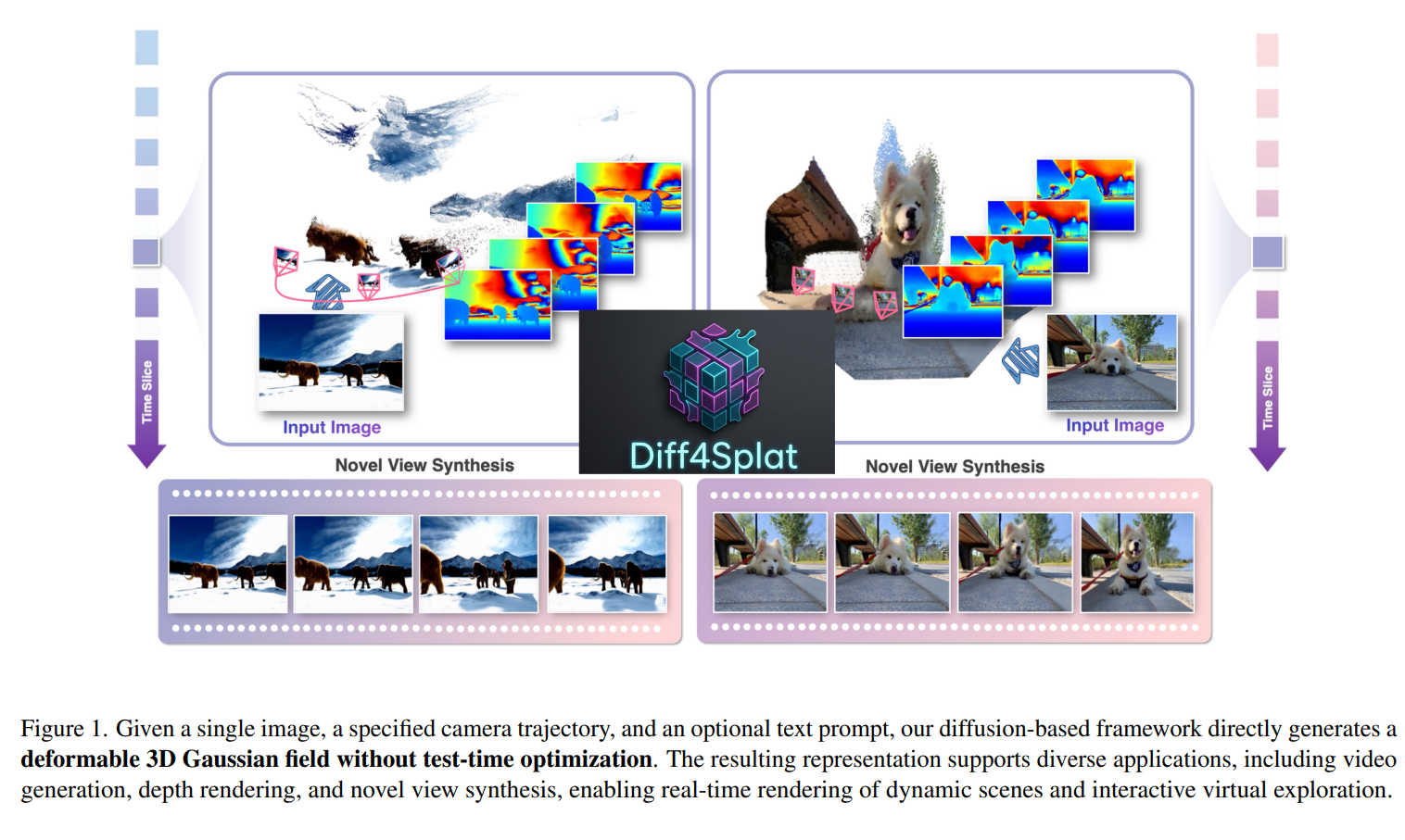
Introduction

기존 video diffusion model 연구는 고품질이면서 시간적으로 일관된 영상을 생성하는 방향으로 빠르게 발전했다. RGB image, depth map, motion trajectory, semantic map 등 다양한 조건을 활용해 생성 결과를 세밀하게 제어하는 방법들이 제안되어 왔다.

이후 camera motion control까지 확장되면서 predefined motion category, LoRA, camera extrinsic, Plücker coordinate 등을 이용하는 방식들이 등장했지만, 복잡한 장면에서는 camera control 정확도가 떨어지거나 특정 class에 종속되는 한계가 있었다.

더 근본적으로는 대부분의 방법이 결과를 2D video frame sequence로만 생성하기 때문에, 장면의 명시적인 3D geometry와 temporal motion을 함께 표현하는 4D representation으로 직접 연결되지 못한다는 문제가 남아 있다.

한편 3D scene generation은 NeRF와 3D Gaussian Splatting 같은 3D representation의 발전과 함께, layout/scene graph 기반의 구조적 생성에서 text나 single image를 조건으로 하는 open-world generation까지 확장되어 왔다.

최근에는 video diffusion의 spatio-temporal prior를 이용해 3D consistency를 높이거나 dynamic 3D/4D scene을 생성하려는 연구도 활발하지만, 기존 dynamic scene 방법들은 multi-view image나 input video를 추가로 요구하는 경우가 많고, monocular video 기반 reconstruction 역시 흔히 per-scene optimization에 의존해 계산 비용이 크다.

최근 feed-forward 방식으로 dynamic pointmap을 직접 예측하는 연구도 등장했지만, 이러한 representation은 photorealistic rendering에서 hole이나 artifact가 발생하기 쉽다는 한계가 있으며, 따라서 빠른 생성과 explicit dynamic 3D representation을 동시에 만족시키는 것이 여전히 핵심 과제로 남아 있다.

Method & Technical Details

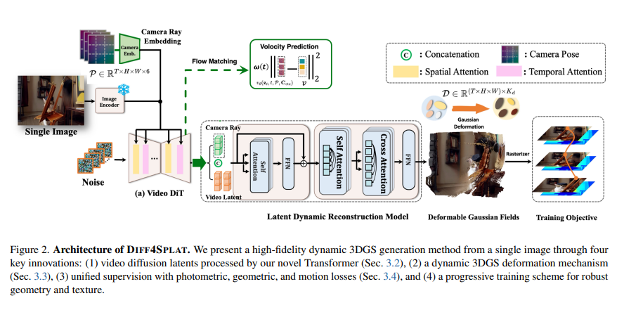
Diff4Splat의 목표는 one single image 한 장으로부터 dynamic 4D scene을 생성하는 것이다. 입력은 크게 세 가지다.

\[I_0 \in \mathbb{R}^{H \times W \times 3}\]

라는 single image, optional text prompt $C_{ctx}$, 그리고 camera trajectory를 나타내는

\[P \in \mathbb{R}^{T \times H \times W \times 6}\]

이다. 여기서 $P$는 각 pixel의 camera ray를 6D Plücker embedding으로 표현한 것이다. 즉 생성될 video가 어떤 camera motion을 따라야 하는지를 모델에 직접 condition으로 넣는다.

전체 흐름은 다음과 같다:

\[\boxed{ \begin{aligned} &I_0,\; P,\; C_{\mathrm{ctx}} \\ &\downarrow \\ &\text{Pre-trained Video Diffusion Model} \\ &\downarrow \\ &\text{Video Latent } z \\ &\downarrow \\ &\text{LDRM} \\ &\begin{cases} \text{Gaussian Geometry / Attributes} \\ \text{Motion / Deformation} \end{cases} \\ &\downarrow \\ &\text{Deformable 3D Gaussian Field} \\ &\downarrow \\ &\text{Dynamic 4D Scene} \end{aligned} }\]

먼저 pretrained video diffusion model이 입력 image와 camera condition을 바탕으로

\[z \in \mathbb{R}^{n \times h \times w \times c}\]

형태의 video latent를 만든다. 이 latent에는 appearance 뿐 아니라 temporal information과 camera 변화에 따른 scene information이 들어가도록 학습된다.

그 다음 LDRM이 이 latent와 camera condition을 받아서 deformable Gaussian field를 예측한다.

이는 기존의 방식들 처럼 “video 생성 후, 별도의 3D reconstruction” 하는 것이 아니라

“video latent를 바로 explicit 4D Gaussian representation” 으로 연결하는 것이다.

이 부분이 논문의 가장 큰 구조라고 이해하면 된다.

Data Curation

일반 video diffusion model을 학습하기 위해서는 RGB video만 있어도 되지만, Diff4Splat은 최종적으로

\[\boxed{\text{appearance + 3D geometry + motion}}\]

을 모두 예측해야 한다.

그래서 RGB frame만 있는 video dataset으로는 부족하며, 각 frame에 대해 metric-scale geometry와 motion annotation이 필요하다.

논문은 이를 위해 synthetic data와 real-world data를 함께 사용한다.

Synthetic dataset

TartanAir, MatrixCity, PointOdyssey, DynamicReplica, Spring, VKITTI2, MultiCamVideo를 사용한다.

Synthetic data의 장점은 renderer 내부에서 scene을 알고 있어 비교적 정확한 Depth, Camera Pose, Geometry, Motion ground truth를 얻을 수 있다는 것이다.

특히 static camera와 moving camera를 모두 포함하기 때문에 모델이 영상에서 보이는 변화가 camera motion 때문인지, object motion 때문인지 구분하는 geometric/dynamic prior를 배우는 데 유용하다.

Real-world dataset

Synthetic data만 사용하면 geometry와 motion GT는 정확하지만 실제 영상의 texture, illumination, object appearance, scene complexity 같은 현실적인 분포를 충분히 학습하기 어렵다.

그래서 저자들은 RealEstate10K와 Stereo4D 같은 real-world data도 사용한다.

그러나 해당 데이터들은 바로 사용하기에는 문제점이 있다. 바로 unknown global scale 문제다.

RealEstate10K의 경우 Camera pose가 존재한다. 이는 COLMAP으로 추정한 camera parameter인데, monocular reconstruction에서는 절대적인 scale을 알 수 없다.

예를 들어 실제 장면에서 카메라 이동을 1m, 물체까지의 거리가 5m라고 한다면, COLMAP의 경우에는 카메라 이동을 0.2, 물체 거리를 1.0으로 복원할 수도 있다.

즉, 비율은 같아서 영상에 projection 했을 때는 동일하게 설명이 가능하다.

그래서 COLMAP이 알려주는 것은 대략

장면 내부의 상대적인 3D 구조

이고, 실제로 몇 m 떨어져 있는지와 같은 global scale은 알 수 없다.

그래서 저자들은 Video Depth Anything과 MegaSaM을 이용해서 metric depth와 camera extrinsics를 다시 추정한다고 설명한다.

목적은

frame마다 제각각인 상대적인 geometry가 아니라, 서로 정렬된 metric-scale geometry를 얻는 것.

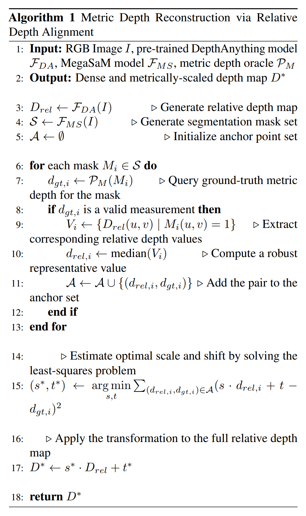
Algorithm 1만 단순화하면,

먼저 DepthAnything에서

\[D_{rel} = \begin{cases} human : 4 \\ sofa: 7 \\ wall: 10 \end{cases}\]

이라는 relative depth map을 얻고, metric depth oracle 이라는 별도의 기준으로부터 일부 영역의 실제 거리 기준값을 얻는다:

\[D_{metric} = \begin{cases} human : 2.0 m\\ sofa: 3.5 m\\ wall: 5.0 m \end{cases}\]

이제 모델 입장에서는 relative depth 값을 어떻게 변환하면 metric depth 값에 가장 잘 맞을지를 푼다:

\[d_{metric} = sd_{rel} + t\]

이렇게 여러 anchor에 가장 잘 맞는 $s,t$를 least squares로 찾고:

\[(s^*, t^*) = arg \underbrace{\text{min}}_{s,t} \sum_{i} (sd_{rel,i} + t - d_{gt, i})^2\]

그 값을 전체 depth map에 적용한다:

\[\boxed{D^* = s^*D_{rel}+t^*}\]

논문은 Algorithm 1에서 metric depth oracle $P_M$을 쓰지만, 그 oracle이 정확히 무엇인지는 본문에서 명확히 설명하지 않는다.

다만 공식 코드에는 RealEstate10K depth를 video-depth-anything + depthPro-scaled 라고 적어 두었다. 그래서 공개 구현 기준으로는 DepthPro가 metric-scale 기준 역할을 하는 것으로 보인다.

해당 두 방식의 preprocessing과 quality filtering을 거쳐 약 130,000 개의 4D training scene을 구축한다.

논문에서는 dynamic object masking과 reprojection-error filtering 같은 quality control도 수행한다고 설명한다.

추가적으로, 여기서 사용된 Video Depth Anything과 MegaSaM이 최종 inference에서 single image를 3D로 lifting하기 위한 외부 module로 들어가지 않는다는 점이 있다.

Latent Dynamic Reconstruction Model

이쯤에서 왜 해당 논문의 저자들은 “video diffusion이 만든 latent를 어떻게 explicit 3D Gaussian representation으로 바꾸는가”에 대한 궁금증이 생길 수 있다.

물론, 그와 더해 굳이 LDRM이 필요한지에 대한 의문점도 생긴다.

일반적인 video diffusion model은 latent 안에 appearance와 temporal information을 잘 담지만, 그 latent 자체가

\[(x,y,z)\]

를 가진 3D scene representation은 아니다. 게다가 저자들은 일반 video diffusion model에는 explicit camera control이 부족하고, 동적 내용도 3D reconstruction에 바로 쓰기에는 일관되지 않을 수 있다고 지적한다.

그래서 저자들은 Latent Dynamic Reconstruction model(LDRM)을 중간에 둔다고 얘기한다.

먼저, Video diffusion Model이 latent $z$를 만든다. 입력은 앞에서 말했던 것처럼

\[I_0, P, C_{ctx}\]

이고, pretrained video diffusion model이 camera pose에 condition되어 latent tensor

\[z \in \mathbb{R}^{n \times h \times w \times c}\]

를 생성한다. 중요한 건 RGB video를 먼저 완성하는 것이 아니라 latent 단계에서 바로 reconstruction branch로 넘긴다는 점이다.

논문은 latent $z$와 camera pose로부터 동일한 길이의 token sequence를 만든 뒤 둘을 concatenate한다고 한다.

\[Z = [z_1, z_2, ... , z_N]\]

라는 latent token들이 있고, 각각에 대응하는 camera 정보

\[P = [p_1, p_2, ... , p_N]\]

를 만든다고 보면 된다. 그리고,

\[[z_i ; p_i]\]

처럼 latent feature와 camera feature를 함께 Transformer에 전달한다. camera 정보를 같이 넣는 이유는 latent만 보고는 어떤 feature가 어떤 camera ray에서 관찰된 것인지 알기 어렵기 때문이다.

이렇게 만든 token sequence를 Transformer blocks에 통과시킨다. Transformer가 하는 일은 여러 spatial/temporal feature와 camera information의 관계를 통합해서 3D reconstruction에 사용할 수 있는 feature를 만드는 것이다.

\[[Z;P] \rightarrow \text{Transformer} \rightarrow F_{3D-aware}\]

Transformer를 통과한 feature를 lightweight decoder가 받아서 3D Gaussian attribute를 regression한다:

\[G_p = (\mu_p, s_p, q_p, \alpha_p, c_p)\]

마지막으로 3D deconvolution을 통해 Transformer가 낮은 resolution의 latent/token 공간에서 처리한 정보를 다시 source video의 spatial/temporal grid에 대응되는 Gaussian prediction으로 올리는 과정을 수행한다.

Deformable Gaussian Fields

Diff4Splat은 time-dependent deformation을 추가한다. 각 Gaussian $p$에 대해 시간 $t$에서 다음 세 가지 변화를 예측한다.

\[\begin{aligned} \Delta \mu_p^t &\in \mathbb{R}^3 \\ \Delta q_p^t &\in \mathbb{R}^4 \\ \Delta s_p^t &\in \mathbb{R}^3 \end{aligned}\]

각각의 의미는 Gaussian이 얼마나 이동했는지, 얼마나 회전했는지, 크기는 얼마나 변했는지를 나타낸다.

그래서 실제 시간 $t$에서의 Gaussian parameter는

\[\begin{aligned} \mu_p^t &= \mu_p^0 + \Delta \mu_p^t \\ q_p^t &= q_p^0 \otimes \Delta q_p^t\\ s_p^t &= s_p^0 + \Delta s_p^t \end{aligned}\]

로 계산된다. 여기서 $\otimes$는 quaternion multiplication이다.

즉, 새 Gaussian을 매 frame마다 따로 만드는 것이 아니라, base Gaussian을 두고 시간에 따른 deformation을 적용하는 구조다.

LDRM은 두 가지 map을 예측한다. 먼저 Gaussian 자체를 나타내는 feature map:

\[G \in \mathbb{R}^{(T \times H \times W) \times K_g}\]

여기서 $K_g$는 하나의 Gaussian을 표현하는 데 필요한 parameter dimension이다. 동시에 deformation map도 예측한다:

\[D \in \mathbb{R}^{(T \times H \times W) \times K_d}\]

그리고 $K_d = 10$이다. 왜냐하면 앞서 position, quaternion, scale parameter의 dimension을 다 더하면 10이 되기 때문이다.

LDRM이 매우 많은 Gaussian을 예측할 수 있기 때문에, opacity가 거의 0인 Gaussian은 사실상 rendering에 기여하지 않는다.

그래서 논문은 $\tau_{opacity} = 0.005$보다 opacity가 작은 Gaussian을 제거한다. 이 pruning은 training과 inference 모두에서 사용한다고 설명한다.

Training Objective

핵심은

Video diffusion backbone은 4D에 적합한 latent를 만들도록 학습하고, LDRM/Gaussian branch는 그 latent로부터 실제 appearance, geometry, motion을 가진 4DGS를 만들도록 학습

이다.

전체 loss는

\[\mathcal{L} = \mathcal{L}_{FM} + \lambda_{photo}\mathcal{L}_{photo} + \lambda_{geo}\mathcal{L}_{geo} + \lambda_{motion}\mathcal{L}_{motion}\]

여기서 $\lambda_{photo} = 1.0, \lambda_{geo} = 0.5, \lambda_{motion} = 2.0$ 으로 설정한다.

Flow Matching Loss

먼저, Flow Matching Loss 인 $L_{FM}$은 3DGS를 직접 학습시키는 loss가 아니다. 이 loss는 base video diffusion model에만 적용된다. 저자들은 pretrained video diffusion model을 그대로 쓰는 것이 아닌, 앞에서 만든 4D-annotated dataset에 맞게 fine-tuning한다.

Flow Matching의 기본 구조는

\[z^{(0)}\]

이라는 clean video latent와

\[z^{(1)} \sim \mathcal{N}(0,I)\]

라는 noise 사이의 경로를 생각하고, 모델이 올바른 velocity/vector field를 예측하도록 하는 것이다.

\[L_{FM}(\theta) = \mathbb{E}_{t,p_t(z^{(t)})} [\lVert v_{\theta}(z^{(t), t}) - u_t(z^{(t)}) \rVert _2^2]\]

여기서 $v_{\theta}$는 diffusion model이 예측한 vector field, $u_t$는 target vector field를 의미한다.

즉, Noise를 통해 4D-consistent video latent를 얻도록 video diffusion backbone을 적응시키는 loss다.

논문에서는

LDRM과 Gaussian prediction head는 FM loss로 학습하지 않고, rendering-based loss들로 학습한다.

라고 표현한다.

Photometric Loss

이제 실제로 Gaussian을 만들어서 target camera에서 rendering한다고 해보자. 예측된 3DGS를 view $k$에서 rendering한 image를

\[\hat{I}_k\]

GT image를

\[I_k\]

라고 한다. 그 둘이 비슷하도록

\[L_{photo} = MSE(\hat{I}_k, I_k) + \lambda_p LPIPS(\hat{I}_k, I_k)\]

를 사용한다. 여기서 MSE는 pixel-by-pixel 차이를 줄인다. 반면 LPIPS는 deep feature를 기반으로 perceptual similarity를 비교해서, texture, 구조 등이 비슷하도록 만든다.

Geometric Loss

Photometric loss만 있으면 RGB가 비슷하게 보이는 3D 구조를 만들 수는 있지만, 그 3D geometry가 반드시 정확하다는 보장이 없다.

예를 들어 같은 image를 render할 수 있는 서로 다른 depth configuration이 존재할 수 있다.

그래서 rendered depth와 GT depth를 직접 비교한다.

예측 Gaussian을 rendering해서 얻은 depth가

\[\hat{D}_k\]

GT depth가

\[D_k^*\]

라고 하면 논문은

\[L_{geo} = 1 - \frac{Cov(\hat{D}_k, D_k^*)}{\sqrt{Var(\hat{D}_k)Var(D_k^*)}}\]

형태의 correlation-based loss를 사용한다. 분수 부분은 사실상 두 depth map 사이의 correlation coefficient라고 보면 된다.

예측 depth와 GT depth의 구조가 잘 맞으면

\[Corr \approx 1\]

이므로

\[L_{geo} \approx 0\]

이 된다.

저자들은 여기에

\[L_{TV} = \lVert \Delta \hat{D}_k \rVert _1\]

도 적용한다. 이건 인접 pixel의 depth가 이유 없이 심하게 튀는 것을 억제한다. 예를 들어 평평한 벽인데 depth가 갑자기 튀면 좋지 않은데, TV loss는 이런 local noise를 줄여서 smooth한 geometry를 유도한다.

Motion Loss

3D point $j$의 GT displacement를

\[\Delta x_j\]

라고 하고, 모델이 예측한 displacement를

\[\Delta \hat{x}_j\]

라고 한다. 그러면

\[L_{motion} = \frac{1}{| \mathcal{O} |} \sum_{j \in \mathcal{O}} (\lambda_m \lVert \Delta \hat{x}_j - \Delta x_j \rVert_2 + \lVert \Delta \hat{x}_j \rVert_1)\]

을 사용한다. 여기서 $\mathcal{O}$는 유효한 tracked point들의 집합이다.

첫 번째 항은 예측한 Gaussian motion이 실제 3D point motion을 따라가라는 의미이고, 두 번째 항은 필요 이상으로 Gaussian을 크게 움직이지 말라는 regularization 역할을 수행한다.

해당 loss들의 의미를 알았다면 다음으로 봐야할 것은 학습 순서다. 저자들은 처음부터 Dynamic 4D scene을 한꺼번에 학습하지 않는다. 총 3단계로 진행한다.

먼저 static scene만을 사용한다. TartanAir, RealEstate10K 등을 사용한다. 그리고 photometric + geometric loss를 사용하고 deformation module은 freeze한다. 여기서는 $256 \times 256$의 resolution을 사용한다.

즉, 먼저 제대로 된 static 3D scene부터 만드는 것을 학습한 후 High-Resolution Refinement를 진행한다. 여기서는 전의 해상도를 $512 \times 512$ resolution으로 올려서 학습하고, 여전히 deformation module은 freeze 상태로 둔다.

이제 마지막으로 deformation module을 unfreeze하고 학습을 진행한다. 사용할 dataset은 PointOdyssey, DynamicReplica, Spring, VKITTI2, Stereo4D이다. full loss를 사용하여 진행한다.

저자들은

직접 dynamic training을 시작하면 3DGS 초기화가 불안정하고 품질이 떨어진다

고 주장하며 ablation에서도 progressive training이 더 안정적이고 효율적이라고 설명한다.

Experiments

Implementation Details

CogVideoX를 video diffusion backbone으로 사용한다. 학습은 AdamW로 100K iterations 진행하며, 32장의 A100 GPU에서 약 7일이 걸리고, inference 시 하나의 dynamic scene 생성에는 약 30초가 소요된다.

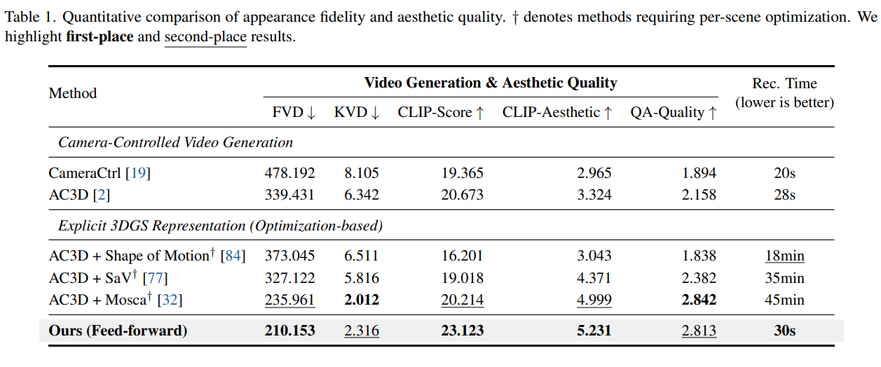
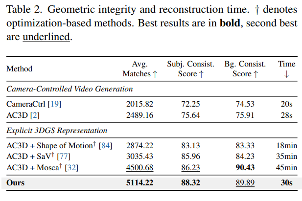
Table 1과 Table 2에서 Diff4Splat이 video quality, aesthetic quality, geometric consistency 측면에서 기존 방법들과 경쟁력 있거나 더 좋은 성능을 보이면서, reconstruction 시간을 약 30초로 크게 줄였다고 보고한다.

특히 Table 2에서는 camera-controllable generation과 geometric integrity 측면에서 강한 성능을 보인다.

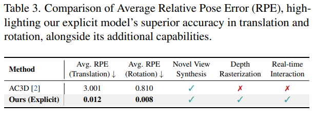
Table 3에서는 Average RPE를 통해 explicit 4D representation이 camera pose를 더 정확하게 따르며, novel view synthesis, depth rasterization, real-time interaction 같은 기능도 지원함을 보여준다.

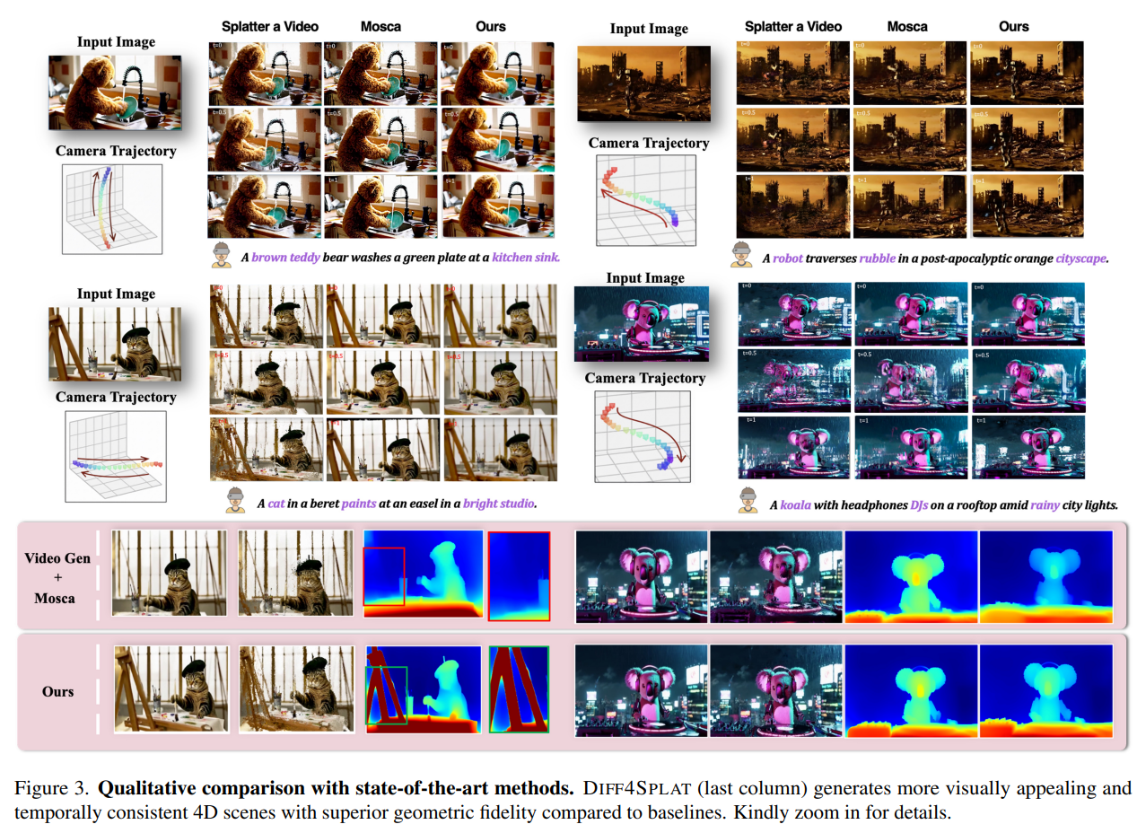
Figure 3에서 SaV, Mosca 등의 baseline보다 더 자연스럽고 temporally coherent하며 geometry artifact가 적은 결과를 제시한다.

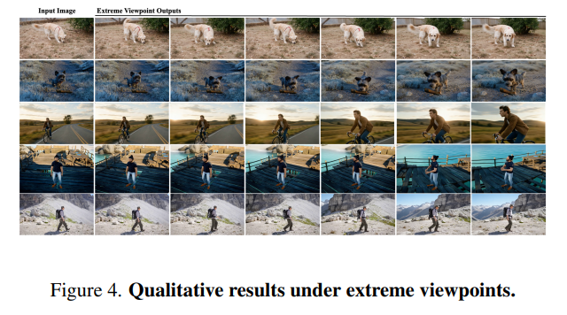
Figure 4에서는 extreme viewpoint 에서도 비교적 안정적인 장면 생성을 보여준다. 또한 저자들은 explicit deformable 3D Gaussian representation 덕분에 지정된 camera path를 deterministic하게 따를 수 있다는 점을 강조한다.

Ablation and Analysis

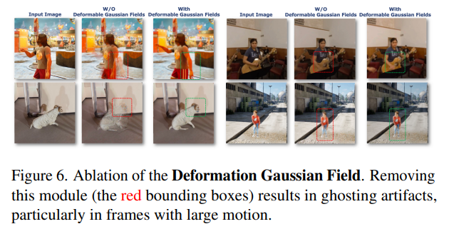
Figure 6에서는 Deformation Gaussian Field를 제거하면 camera motion과 foreground object motion을 제대로 분리하지 못해 ghosting, motion blur, spike artifact가 발생함을 보여준다.

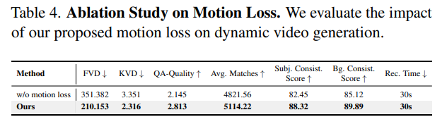
Table 4에서는 motion loss를 제거할 경우 FVD, KVD, QA-Quality뿐 아니라 Avg.Matches와 subject/background consistency까지 모두 악화되어, 3D motion supervision이 temporal deformation 학습에 중요함을 확인한다.

또한 Table 3을 통해 explicit 3DGS representation이 낮은 RPE와 함께 depth rasterization, novel-view synthesis, real-time interaction 같은 기능적 장점을 제공함을 강조한다.

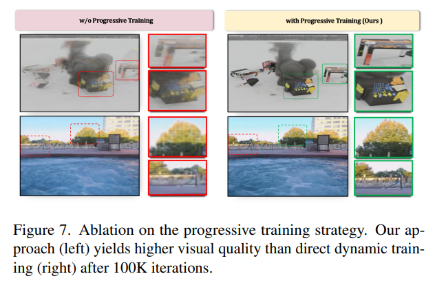
Figure 7에서는 static geometry를 먼저 학습한 뒤 dynamic fine-tuning으로 넘어가는 progressive training이 처음부터 dynamic scene을 직접 학습하는 방식보다 더 안정적이고 높은 visual quality를 보이며, 학습 시간 측면에서도 더 효율적이라고 분석한다.

Contributions

• Diffusion model이 한 번의 forward pass 만으로 deformable 3D Gaussian field를 직접 생성하도록 해, per-scene optimization 없이 explicit 4D scene을 생성한다.
• latent에서 직접 deformable 3D Gaussian representation을 예측한다.
• Metric-scale geometry와 motion annotation을 포함한 대규모 4D training dataset을 구축한다.
• single image에서 high-fidelity dynamic 3D scene을 생성하며, 기존 복잡한 two-stage pipeline보다 quality와 efficiency 모두에서 우수함을 실험적으로 보인다.

Limitations & Future work

해당 저자들은 따로 limitation이나 future work를 제공하지 않는다. 해당 논문은 inference 생성에서 30초 만에 Dynamic Scene을 만드는 좋은 novelty를 만들어냈다고 생각한다.

그러나 interaction이 충분할 만큼의 inference 속도를 지니고 있지 않으며, 추가로 저자들이 구축한 대규모 4D dataset이 빨리 공개되어 다른 연구자들의 future research에 도움이 되길 바란다.