[Paper Review, EN] Diff4Splat: Repurposing Video Diffusion Models for Dynamic Scene Generation
Paper Information
Title: Diff4Splat: Repurposing Video Diffusion Models for Dynamic Scene Generation
Authors: Panwang Pan, Chenguo Lin, Jingjing Zhao, Chenxin Li, Yuchen Lin, Haopeng Li, Honglei Yan, Kairun Wen, Yunlong Lin, Yixuan Yuan, Yadong Mu
Venue: CVPR 2026
Link: [Paper], [Project], [GitHub]
Teaser Image
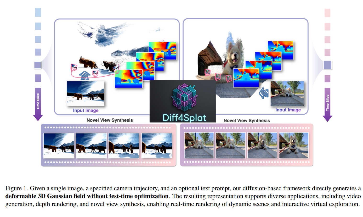
Introduction
Existing video diffusion model research has rapidly advanced toward generating high-quality and temporally consistent videos. Various methods have been proposed to achieve fine-grained control over generation results using diverse conditions such as RGB images, depth maps, motion trajectories, and semantic maps.
As research later expanded to camera motion control, approaches using predefined motion categories, LoRA, camera extrinsics, and Plücker coordinates emerged. However, they still suffered from limitations such as reduced camera-control accuracy in complex scenes or dependence on specific classes.
More fundamentally, most methods generate only 2D video frame sequences, leaving a gap between video generation and a direct 4D representation that jointly captures explicit 3D geometry and temporal motion.
Meanwhile, with the development of 3D representations such as NeRF and 3D Gaussian Splatting, 3D scene generation has expanded from structured generation based on layouts or scene graphs to open-world generation conditioned on text or a single image.
Recently, research has also actively explored leveraging the spatio-temporal priors of video diffusion to improve 3D consistency or generate dynamic 3D/4D scenes. However, existing dynamic-scene methods often require additional multi-view images or input videos, while monocular-video-based reconstruction commonly relies on computationally expensive per-scene optimization.
Recent feed-forward methods have also attempted to directly predict dynamic pointmaps, but such representations are prone to holes or artifacts in photorealistic rendering. Therefore, achieving both fast generation and an explicit dynamic 3D representation remains a key challenge.
Method & Technical Details
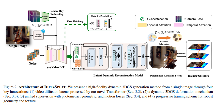
The goal of Diff4Splat is to generate a dynamic 4D scene from a single image. The input consists of three main components.
\[I_0 \in \mathbb{R}^{H \times W \times 3}\]a single image, an optional text prompt $C_{ctx}$, and
\[P \in \mathbb{R}^{T \times H \times W \times 6}\]which represents the camera trajectory. Here, $P$ represents the camera ray of each pixel as a 6D Plücker embedding. In other words, the camera motion that the generated video should follow is directly provided to the model as a condition.
The overall pipeline is as follows:
\[\boxed{ \begin{aligned} &I_0,\; P,\; C_{\mathrm{ctx}} \\ &\downarrow \\ &\text{Pre-trained Video Diffusion Model} \\ &\downarrow \\ &\text{Video Latent } z \\ &\downarrow \\ &\text{LDRM} \\ &\begin{cases} \text{Gaussian Geometry / Attributes} \\ \text{Motion / Deformation} \end{cases} \\ &\downarrow \\ &\text{Deformable 3D Gaussian Field} \\ &\downarrow \\ &\text{Dynamic 4D Scene} \end{aligned} }\]First, the pretrained video diffusion model takes the input image and camera condition to produce
\[z \in \mathbb{R}^{n \times h \times w \times c}\]a video latent of this form. This latent is trained to contain not only appearance information but also temporal information and scene information induced by camera changes.
Next, the LDRM takes this latent together with the camera condition and predicts a deformable Gaussian field.
Unlike existing approaches that “generate a video and then perform separate 3D reconstruction,” Diff4Splat
“directly maps the video latent to an explicit 4D Gaussian representation.”
This can be understood as the core structure of the paper.
Data Curation
Although RGB video alone is sufficient to train a general video diffusion model, Diff4Splat ultimately needs to predict
\[\boxed{\text{appearance + 3D geometry + motion}}\]all of these components.
Therefore, a video dataset containing only RGB frames is insufficient; metric-scale geometry and motion annotations are required for each frame.
To this end, the paper uses both synthetic data and real-world data.
Synthetic dataset
The authors use TartanAir, MatrixCity, PointOdyssey, DynamicReplica, Spring, VKITTI2, and MultiCamVideo.
The advantage of synthetic data is that the renderer has access to the underlying scene, allowing relatively accurate Depth, Camera Pose, Geometry, and Motion ground truth to be obtained.
In particular, because the datasets contain both static and moving cameras, they are useful for learning geometric/dynamic priors that help the model distinguish whether observed changes in a video come from camera motion or object motion.
Real-world dataset
Using only synthetic data provides accurate geometry and motion GT, but it is difficult to sufficiently learn realistic distributions such as texture, illumination, object appearance, and scene complexity found in real videos.
Therefore, the authors also use real-world data such as RealEstate10K and Stereo4D.
However, these datasets cannot be used directly because of the unknown global scale problem.
RealEstate10K provides camera poses estimated by COLMAP, but the absolute scale cannot be recovered from monocular reconstruction.
For example, suppose that in the real scene the camera moves by 1 m and an object is 5 m away. COLMAP may instead reconstruct the camera motion as 0.2 and the object distance as 1.0.
The ratios are the same, so both reconstructions can explain the same image projections.
Thus, what COLMAP provides is roughly
the relative 3D structure within the scene
and it cannot determine the global scale, such as how many meters away an object actually is.
Therefore, the authors explain that they re-estimate metric depth and camera extrinsics using Video Depth Anything and MegaSaM.
The goal is
to obtain metric-scale geometry aligned across frames, rather than relative geometry that varies independently from frame to frame.
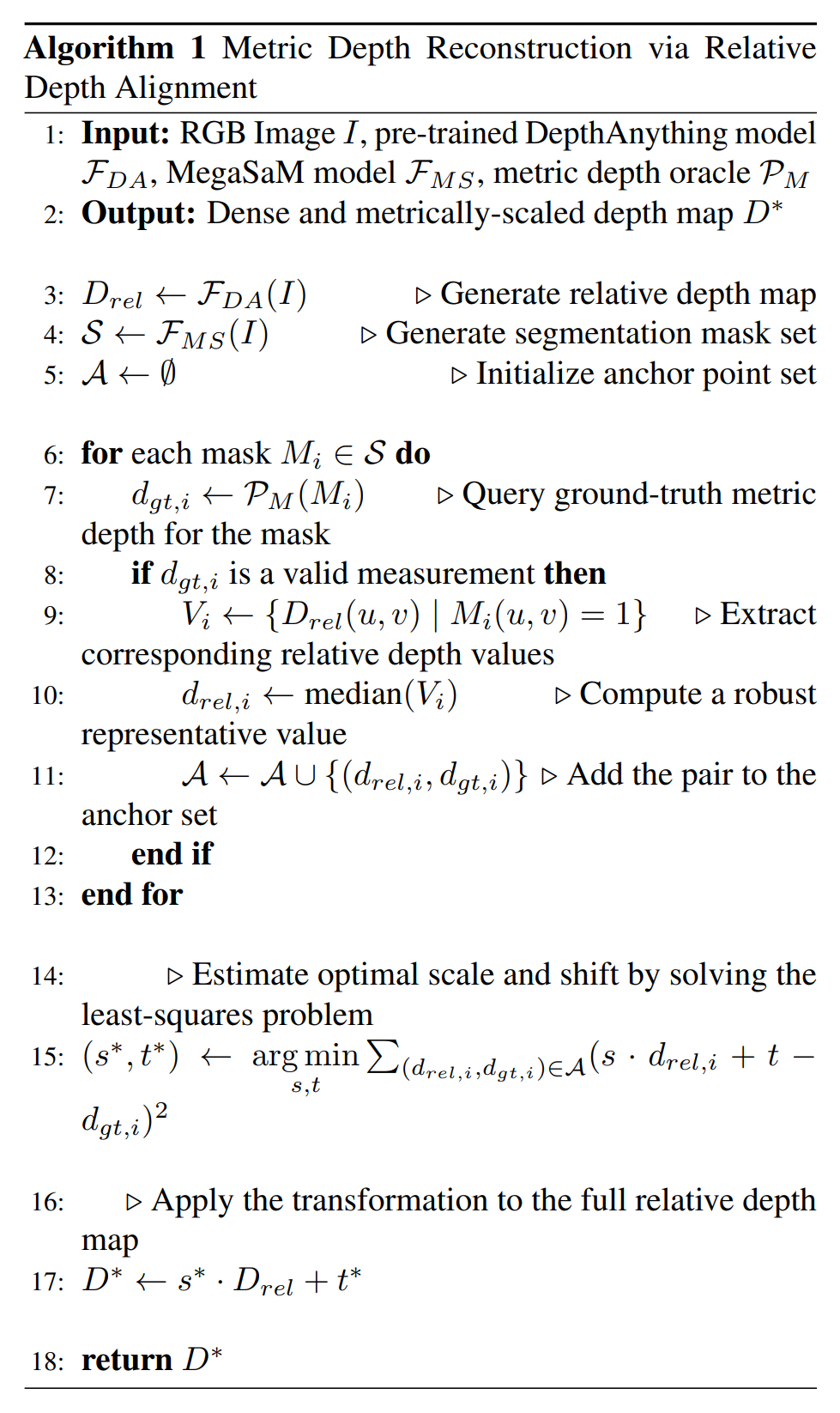
A simplified version of Algorithm 1 is as follows.
First, DepthAnything produces
\[D_{rel} = \begin{cases} human : 4 \\ sofa: 7 \\ wall: 10 \end{cases}\]as the relative depth map, while a separate metric depth oracle provides actual distance references for selected regions:
\[D_{metric} = \begin{cases} human : 2.0 m\\ sofa: 3.5 m\\ wall: 5.0 m \end{cases}\]The model then solves for how the relative depth values should be transformed to best match the metric depth values:
\[d_{metric} = sd_{rel} + t\]It finds the $s,t$ values that best fit multiple anchors using least squares:
\[(s^*, t^*) = arg \underbrace{\text{min}}_{s,t} \sum_{i} (sd_{rel,i} + t - d_{gt, i})^2\]and applies those values to the entire depth map:
\[\boxed{D^* = s^*D_{rel}+t^*}\]Algorithm 1 uses a metric depth oracle $P_M$, but the paper does not clearly explain what this oracle specifically is.
However, the official code describes the RealEstate10K depth as video-depth-anything + depthPro-scaled. Therefore, based on the released implementation, DepthPro appears to serve as the metric-scale reference.
Through preprocessing and quality filtering of these two data sources, the authors construct approximately 130,000 4D training scenes.
The paper also describes quality-control procedures such as dynamic object masking and reprojection-error filtering.
Another important point is that Video Depth Anything and MegaSaM, which are used here, are not external modules used to lift a single image into 3D during final inference.
Latent Dynamic Reconstruction Model
At this point, one may wonder “how the latent generated by video diffusion is converted into an explicit 3D Gaussian representation.”
It is also natural to ask why an LDRM is needed in the first place.
A typical video diffusion model captures appearance and temporal information well in its latent space, but the latent itself is not a 3D scene representation with
\[(x,y,z)\]coordinates. In addition, the authors point out that general video diffusion models lack explicit camera control, and their dynamic content may be insufficiently consistent for direct use in 3D reconstruction.
For this reason, the authors place a Latent Dynamic Reconstruction Model (LDRM) between the video diffusion model and the Gaussian representation.
First, the video diffusion model generates the latent $z$. As described earlier, its inputs are
\[I_0, P, C_{ctx}\]and the pretrained video diffusion model is conditioned on the camera pose to generate the latent tensor
\[z \in \mathbb{R}^{n \times h \times w \times c}\]The important point is that the model does not first complete an RGB video; instead, it passes the latent directly to the reconstruction branch.
The paper states that it creates latent tokens and camera-pose tokens of identical sequence length from the latent $z$ and the camera pose, and then concatenates them.
\[Z = [z_1, z_2, ... , z_N]\]Here, the latent tokens are
\[P = [p_1, p_2, ... , p_N]\]and the corresponding camera information is constructed as shown above. Then,
\[[z_i ; p_i]\]the latent feature and camera feature are jointly passed to the Transformer. The camera information is included because, from the latent alone, it is difficult to determine which feature was observed along which camera ray.
The resulting token sequence is passed through Transformer blocks. The role of the Transformer is to integrate relationships among spatial/temporal features and camera information into features suitable for 3D reconstruction.
\[[Z;P] \rightarrow \text{Transformer} \rightarrow F_{3D-aware}\]A lightweight decoder then takes the Transformer output features and regresses the 3D Gaussian attributes:
\[G_p = (\mu_p, s_p, q_p, \alpha_p, c_p)\]Finally, 3D deconvolution upsamples the information processed by the Transformer in the low-resolution latent/token space into Gaussian predictions corresponding to the spatial/temporal grid of the source video.
Deformable Gaussian Fields
Diff4Splat adds time-dependent deformation. For each Gaussian $p$, it predicts the following three types of changes at time $t$.
\[\begin{aligned} \Delta \mu_p^t &\in \mathbb{R}^3 \\ \Delta q_p^t &\in \mathbb{R}^4 \\ \Delta s_p^t &\in \mathbb{R}^3 \end{aligned}\]These respectively represent how much the Gaussian moves, rotates, and changes in scale.
Thus, the Gaussian parameters at actual time $t$ are
\[\begin{aligned} \mu_p^t &= \mu_p^0 + \Delta \mu_p^t \\ q_p^t &= q_p^0 \otimes \Delta q_p^t\\ s_p^t &= s_p^0 + \Delta s_p^t \end{aligned}\]computed as above, where $\otimes$ denotes quaternion multiplication.
In other words, instead of creating a separate new Gaussian for every frame, the model maintains a base Gaussian and applies time-dependent deformations to it.
The LDRM predicts two maps. The first is a feature map representing the Gaussian itself:
\[G \in \mathbb{R}^{(T \times H \times W) \times K_g}\]Here, $K_g$ is the parameter dimension required to represent a single Gaussian. At the same time, the model also predicts a deformation map:
\[D \in \mathbb{R}^{(T \times H \times W) \times K_d}\]Here, $K_d = 10$ because the dimensions of the position, quaternion, and scale parameters sum to 10.
Because the LDRM can predict a very large number of Gaussians, Gaussians with near-zero opacity contribute almost nothing to rendering.
Therefore, the paper removes Gaussians whose opacity is below $\tau_{opacity} = 0.005$. This pruning is applied during both training and inference.
Training Objective
The key idea is
The video diffusion backbone is trained to produce latents suitable for 4D, while the LDRM/Gaussian branch is trained to convert those latents into a 4DGS representation with actual appearance, geometry, and motion.
This is the central training principle.
The total loss is
\[\mathcal{L} = \mathcal{L}_{FM} + \lambda_{photo}\mathcal{L}_{photo} + \lambda_{geo}\mathcal{L}_{geo} + \lambda_{motion}\mathcal{L}_{motion}\]where $\lambda_{photo} = 1.0, \lambda_{geo} = 0.5, \lambda_{motion} = 2.0$.
Flow Matching Loss
First, the Flow Matching Loss $L_{FM}$ is not a loss that directly trains the 3DGS. It is applied only to the base video diffusion model. Rather than using the pretrained video diffusion model as-is, the authors fine-tune it on the 4D-annotated dataset constructed earlier.
The basic Flow Matching formulation starts with
\[z^{(0)}\]as a clean video latent and
\[z^{(1)} \sim \mathcal{N}(0,I)\]as noise, and trains the model to predict the correct velocity/vector field along the path between them.
\[L_{FM}(\theta) = \mathbb{E}_{t,p_t(z^{(t)})} [\lVert v_{\theta}(z^{(t), t}) - u_t(z^{(t)}) \rVert _2^2]\]Here, $v_{\theta}$ denotes the vector field predicted by the diffusion model, while $u_t$ denotes the target vector field.
In other words, this loss adapts the video diffusion backbone so that it produces 4D-consistent video latents from noise.
The paper states that
the LDRM and Gaussian prediction head are not trained with the FM loss; they are trained with rendering-based losses.
This is how the paper describes the separation of the training objectives.
Photometric Loss
Now suppose that the predicted Gaussians are rendered from a target camera. Let the image rendered from the predicted 3DGS at view $k$ be
\[\hat{I}_k\]and the GT image be
\[I_k\]The following loss is used to make the two images similar:
\[L_{photo} = MSE(\hat{I}_k, I_k) + \lambda_p LPIPS(\hat{I}_k, I_k)\]Here, MSE reduces pixel-by-pixel differences. In contrast, LPIPS compares perceptual similarity based on deep features, encouraging similar texture and structure.
Geometric Loss
With only the photometric loss, the model can produce a 3D structure that renders RGB images similarly, but there is no guarantee that the underlying 3D geometry is actually correct.
For example, multiple different depth configurations may render the same image.
Therefore, the rendered depth is directly compared with the GT depth.
Let the depth obtained by rendering the predicted Gaussians be
\[\hat{D}_k\]and the GT depth be
\[D_k^*\]Then, the paper uses
\[L_{geo} = 1 - \frac{Cov(\hat{D}_k, D_k^*)}{\sqrt{Var(\hat{D}_k)Var(D_k^*)}}\]a correlation-based loss of this form. The fractional term can essentially be viewed as the correlation coefficient between the two depth maps.
If the structures of the predicted depth and GT depth match well,
\[Corr \approx 1\]then
\[L_{geo} \approx 0\]which means the geometric loss approaches zero.
The authors additionally apply
\[L_{TV} = \lVert \Delta \hat{D}_k \rVert _1\]This suppresses abrupt, unjustified depth changes between neighboring pixels. For example, a flat wall should not exhibit sudden depth jumps; the TV loss reduces such local noise and encourages smoother geometry.
Motion Loss
Let the GT displacement of 3D point $j$ be
\[\Delta x_j\]and the displacement predicted by the model be
\[\Delta \hat{x}_j\]Then, the motion loss is
\[L_{motion} = \frac{1}{| \mathcal{O} |} \sum_{j \in \mathcal{O}} (\lambda_m \lVert \Delta \hat{x}_j - \Delta x_j \rVert_2 + \lVert \Delta \hat{x}_j \rVert_1)\]where $\mathcal{O}$ is the set of valid tracked points.
The first term encourages the predicted Gaussian motion to follow the actual 3D point motion, while the second term acts as a regularizer that discourages unnecessarily large Gaussian motion.
After understanding these losses, the next important aspect is the training schedule. The authors do not train the entire dynamic 4D scene from the beginning; training proceeds in three stages.
First, the model uses only static scenes, including TartanAir and RealEstate10K. It is trained with photometric + geometric losses while the deformation module remains frozen, at a resolution of $256 \times 256$.
After first learning to construct a proper static 3D scene, the model proceeds to High-Resolution Refinement. The resolution is increased to $512 \times 512$, while the deformation module remains frozen.
Finally, the deformation module is unfrozen and training continues on PointOdyssey, DynamicReplica, Spring, VKITTI2, and Stereo4D using the full loss.
The authors argue that
directly starting with dynamic training leads to unstable 3DGS initialization and degraded quality
and explain through the ablation study that progressive training is more stable and efficient.
Experiments
Implementation Details
CogVideoX is used as the video diffusion backbone. The model is trained with AdamW for 100K iterations, requiring approximately 7 days on 32 A100 GPUs, while inference takes about 30 seconds to generate one dynamic scene.
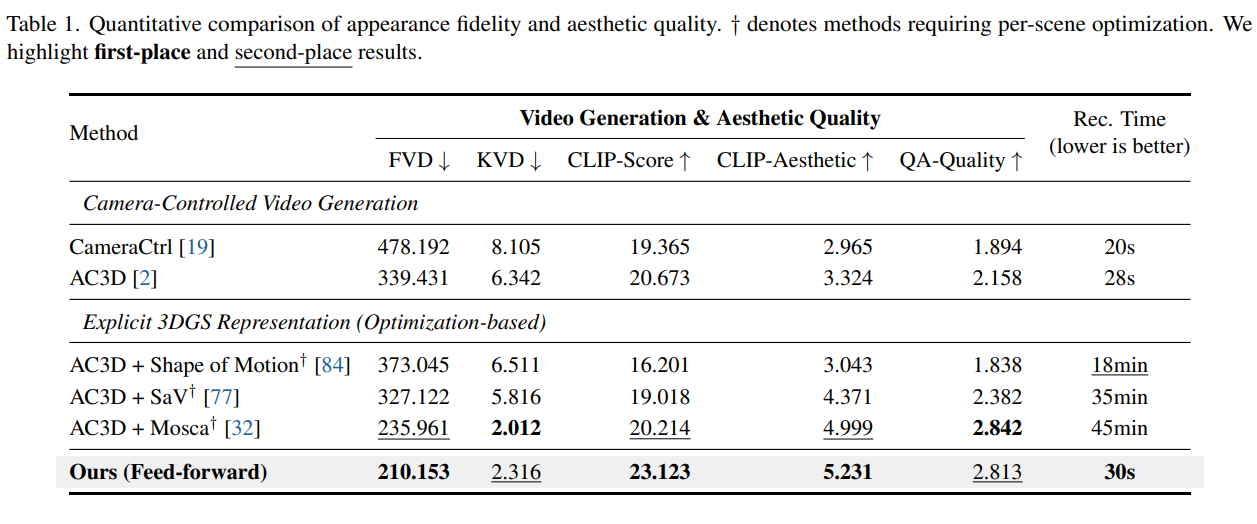
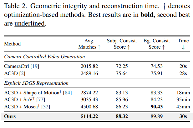
Tables 1 and 2 report that Diff4Splat achieves competitive or better performance than existing methods in terms of video quality, aesthetic quality, and geometric consistency, while substantially reducing reconstruction time to approximately 30 seconds.
In particular, Table 2 shows strong performance in camera-controllable generation and geometric integrity.
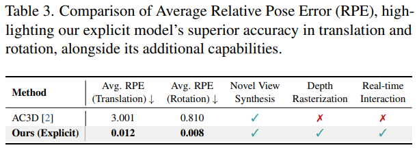
Table 3 shows through Average RPE that the explicit 4D representation follows the camera pose more accurately and also supports functions such as novel view synthesis, depth rasterization, and real-time interaction.
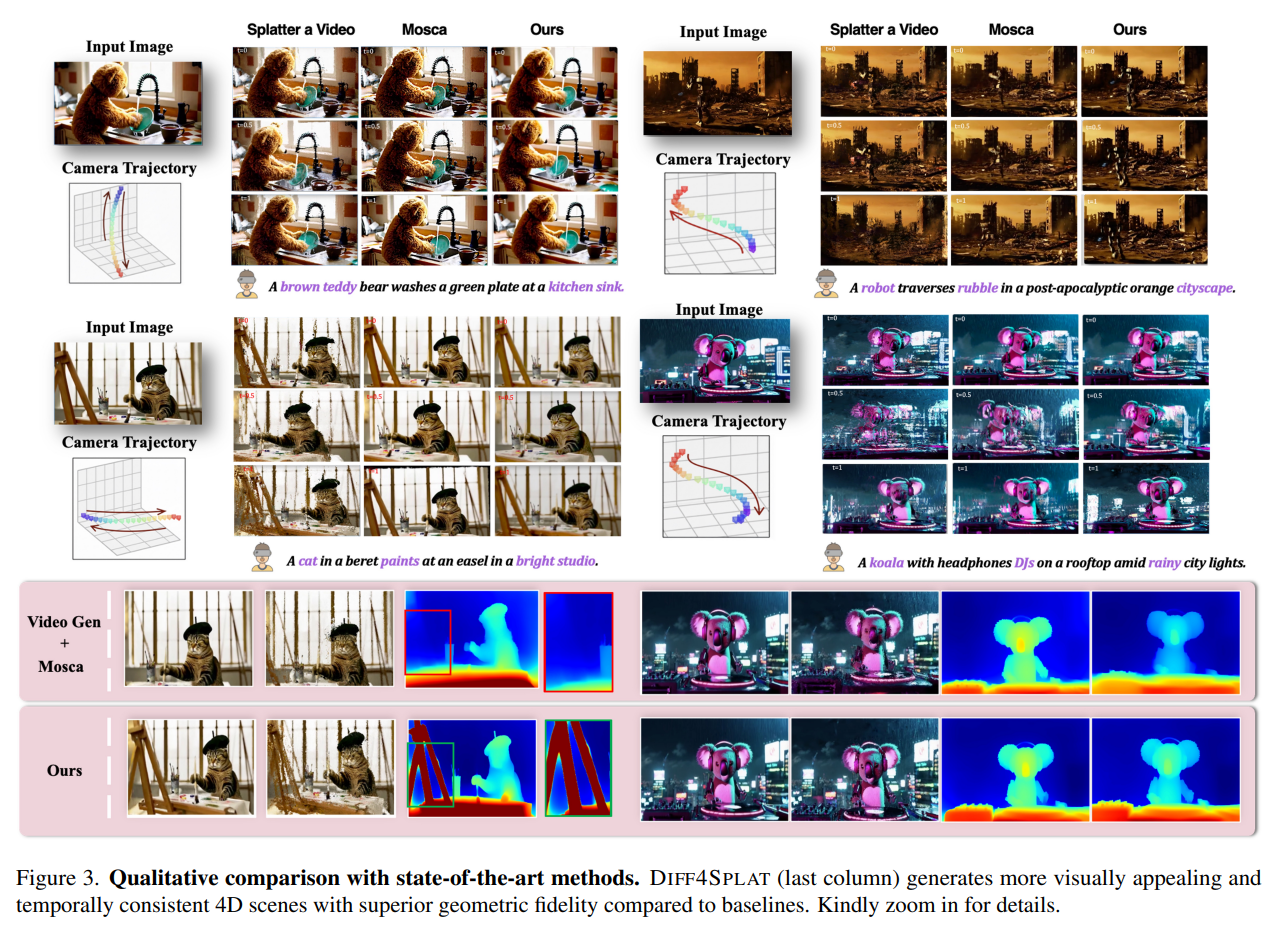
Figure 3 presents results that are more natural, temporally coherent, and contain fewer geometry artifacts than baselines such as SaV and Mosca.
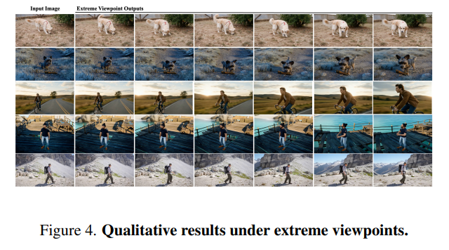
Figure 4 shows relatively stable scene generation even under extreme viewpoints. The authors also emphasize that the explicit deformable 3D Gaussian representation allows the model to deterministically follow a specified camera path.
Ablation and Analysis
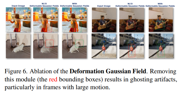
Figure 6 shows that removing the Deformation Gaussian Field prevents the model from properly separating camera motion from foreground object motion, resulting in ghosting, motion blur, and spike artifacts.
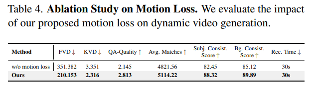
Table 4 shows that removing the motion loss degrades not only FVD, KVD, and QA-Quality but also Avg. Matches and subject/background consistency, confirming that 3D motion supervision is important for learning temporal deformation.
Table 3 further emphasizes that the explicit 3DGS representation provides functional advantages such as depth rasterization, novel-view synthesis, and real-time interaction, together with low RPE.
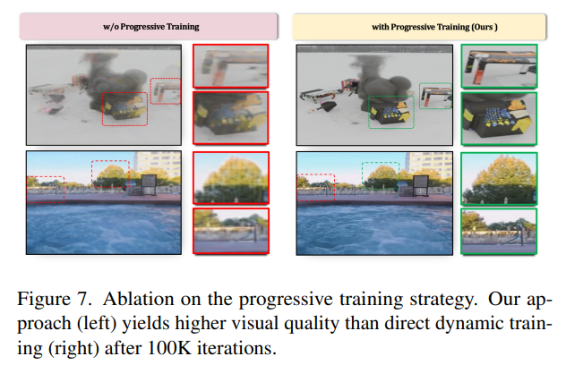
Figure 7 analyzes that progressive training, which first learns static geometry and then proceeds to dynamic fine-tuning, is more stable, produces higher visual quality, and is also more efficient in training time than directly training on dynamic scenes from the beginning.
Contributions
- The diffusion model directly generates a deformable 3D Gaussian field in a single forward pass, enabling explicit 4D scene generation without per-scene optimization.
- It directly predicts a deformable 3D Gaussian representation from the latent.
- It constructs a large-scale 4D training dataset containing metric-scale geometry and motion annotations.
- It generates high-fidelity dynamic 3D scenes from a single image and experimentally demonstrates better quality and efficiency than complex existing two-stage pipelines.
Limitations & Future work
The authors do not provide a separate limitations or future work section. In my view, the paper introduces a compelling novelty by generating a Dynamic Scene in only 30 seconds at inference time.
However, the inference speed is still not fast enough for sufficiently interactive use, and I also hope that the large-scale 4D dataset constructed by the authors will be released soon to support future research by other researchers.