[Paper Review, EN] Turbo3D: Ultra-fast Text-to-3D Generation
Paper Information
Title: Turbo3D: Ultra-fast Text-to-3D Generation
Authors: Hanzhe Hu, Tianwei Yin, Fujun Luan, Yiwei Hu, Hao Tan, Zexiang Xu, Sai Bi, Shubham Tulsiani, Kai Zhang
Venue: CVPR 2025
Link: [Paper], [Project], [GitHub]
Teaser Image
Introduction
In the text-to-image field, inference speed has been greatly improved through techniques such as one-step/few-step generation and diffusion distillation based on diffusion models. In contrast, these advances have not yet been sufficiently carried over to 3D generation.
Existing text-to-3D methods can be broadly divided into optimization-based methods and generative methods. Optimization-based methods can achieve relatively high quality by distilling the prior of a pretrained 2D diffusion model to optimize a 3D representation, but their high inference cost is problematic, as generating a single 3D asset can take from several minutes to several hours.
Meanwhile, early generative methods attempted to directly generate 3D representations such as point clouds or SDFs, but the limited availability of high-quality 3D data for training constrains both generation quality and generalization.
To address this, recent methods commonly first generate text-conditioned multi-view images and then reconstruct them into 3D. However, fine-tuning a multi-view diffusion model on synthetic 3D data can degrade image quality, and the overall text-to-3D pipeline remains slow because diffusion sampling still requires multiple iterative denoising steps.
In addition, prior diffusion distillation studies have mainly focused on 2D image generation, so directly applying them to multi-view diffusion can further exacerbate mode collapse as fine-tuning and distillation consecutively reduce diversity.
Method & Technical Details
Background
Before presenting their method, the authors first introduce the necessary background concepts.
Multi-view Diffusion model
The authors first explain the Multi-view Diffusion Model.
In a standard diffusion model, Gaussian noise is progressively added to a clean sample $x_0$ to obtain $x_t$, and the model is trained to reverse this process by removing the noise. The paper defines the forward noising process as follows:
\[q(x_t | x_0) = \mathcal{N}(x_t; \alpha_t x_0, \sigma_t^2 I)\]Here, $\alpha_t$ indicates how much of the original signal remains, while $\sigma_t$ represents the noise magnitude. The model $\epsilon_{\theta}$ takes $x_t$ and timestep $t$ as inputs and is trained to predict the originally added noise $\epsilon$.
\[\mathcal{L} (\theta) = \mathbb{E}[\lVert \epsilon - \epsilon_{\theta}(x_t, t) \rVert^2]\]This is the standard noise-prediction diffusion training scheme. The paper notes that other parameterizations, such as directly predicting $x_0$ or predicting velocity, are also possible, but Turbo3D adopts the noise prediction formulation.
The paper also explains that these predictions can ultimately be related to the score function of the data distribution
\[s_{\theta}(x_t, t) = \nabla_{x_t} log \; p(x_t)\]as shown above.
While a standard diffusion model denoises a single image $x$, a multi-view diffusion model simultaneously denoises multiple views of the same 3D object.
The paper uses
\[\{x^i\}_{i=1}^K\]$K$ multi-view images represented as above.
The key point is that the views are not generated independently; instead, they are jointly denoised within a single model.
Accordingly, the paper presents the training objective in the following form:
\[\mathbb{E}[\lVert \epsilon - \epsilon_{\theta}(\{x^i\}_{i=1}^K, t, c) \rVert^2]\]Here, $c$ is the text prompt. Importantly, independent Gaussian noise is added to each view, but the model receives all views simultaneously and predicts their noise together.
As a result, the model learns multi-view consistency so that the generated views represent the same 3D object as consistently as possible.
Distribution Matching Distillation(DMD)
The paper describes DMD as a method for distilling a diffusion teacher that requires many denoising steps into a student that can generate samples in far fewer steps.
I have already reviewed this technique in several previous papers.
The key idea is to match the distribution $p_{fake}$ produced by the student generator $G_{\theta}$ to $p_{real}$, which is close to the real data distribution.
This is expressed using reverse KL divergence:
\[L_{DMD}(\theta) = D_{KL}(p_{fake} || p_{real})\]The paper writes this as
\[L_{DMD}(\theta) = \mathbb{E}_{x,t} [log \frac{p_{fake}(x_t)} {p_{real}(x_t)}]\]In other words, the objective of DMD is to move the student-generated distribution $p_{fake}$ toward the Teacher/Data distribution $p_{real}$.
How the distributions themselves are compared is also important.
Because directly computing the probability density of $p_{real}(x)$ or $p_{fake}(x)$ is difficult, DMD instead uses the corresponding score functions.
\[\begin{aligned} s_{real}(x_t, t)&= \nabla_{x_t} log \; p_{real} (x_t) \\ s_{fake} (x_t, t)&= \nabla_{x_t} log \; p_{fake} (x_t) \end{aligned}\]The gradient of the reverse KL divergence is then approximated by the difference between these two scores.
\[\nabla_{\theta} L_{\mathrm{DMD}}(\theta) \approx \mathbb{E}_{z,t} \left[ -w_t \left( s_{\mathrm{real}} \left( F(G_{\theta}(z), t), t \right) - s_{\mathrm{fake}} \left( F(G_{\theta}(z), t), t \right) \right) \frac{dG_{\theta}(z)}{d\theta} \right]\]More precisely, the two scores are evaluated on a noisy sample obtained by applying the forward diffusion process $F(\cdot, t)$ to the student’s generated output.
The student $G_{\theta}$ is updated using this score difference.
Additionally, in the basic one-step DMD setting, the student $G_{\theta}$ can be viewed as taking pure Gaussian noise as input and producing the result in a single step:
\[\epsilon \rightarrow G_{\theta} \rightarrow x_0\]Turbo3D, however, aims to build a 4-step generator. Therefore, the student does not need to map pure noise all the way to a clean image in one step; instead, it can take an intermediate noisy sample $x_t$ from the diffusion process as input and predict a cleaner state.
From this point onward, the paper describes its proposed methods.
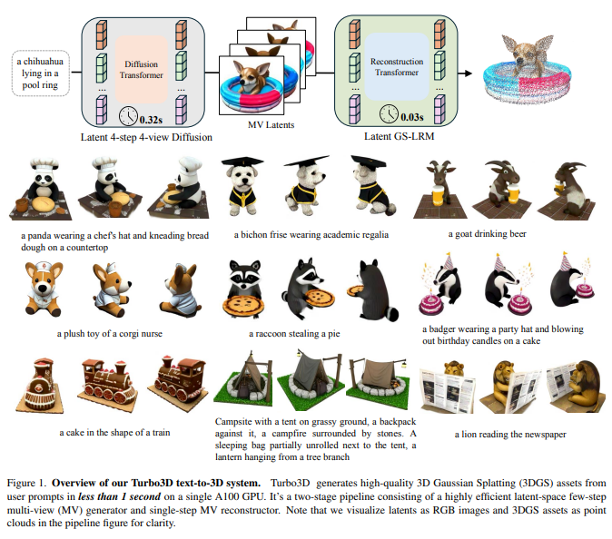
The Turbo3D pipeline consists of two main components: a Few-step Multi-view Generator and a Multi-view Reconstructor. The Few-step Multi-view Generator is trained using Dual-teacher Distillation, while the Multi-view Reconstructor is implemented as Latent GS-LRM.
Dual-teacher Distillation for MV Diffusion
Turbo3D first points out the inefficiency of conventional multi-view diffusion models. When generating multiple views from a text prompt, the denoiser must be evaluated repeatedly, making the MV generation stage itself a major bottleneck in the text-to-3D pipeline.
To reduce this cost, the paper proposes using diffusion distillation, such as DMD/DMD2 described above, to convert a many-step MV diffusion model into a single-step or few-step MV generator.
However, using only a single MV Teacher for distillation causes a problem. The authors observe that
When the student is distilled with DMD using only the MV teacher, its outputs become overly simple and cartoon-like.
This is what the authors observed.
In particular, the outputs become very similar to the style of the synthetic 3D assets in Objaverse, which was used to fine-tune the MV teacher.
The authors call this phenomenon compounding mode collapse. It is called compounding because mode collapse accumulates over two stages rather than occurring only once.
To illustrate this compounding mode collapse process, suppose we start with a powerful text-to-image model. This model has originally learned a broad distribution from internet-scale image data.
When it is fine-tuned on Objaverse multi-view data:
\[p_{original} \rightarrow p_{\text{MV teacher}}\]the distribution narrows toward Objaverse. In other words, the first reduction in diversity has already occurred.
If that MV teacher is then distilled again into a few-step student,
\[P_{text{MV teacher}} \rightarrow p_{student}\]diversity can decrease once more during this process. As a result, the distribution is effectively compressed twice toward the synthetic Objaverse mode.
Now consider how Turbo3D addresses this issue. Turbo3D introduces one additional teacher.
Instead of using only the MV teacher, Turbo3D adds a single-view teacher called the SV teacher. First, the MV teacher teaches multi-view consistency. For example, if there are four views,
\[\{x^1, x^2, x^3, x^4\}\]the four images are considered together as a single set to determine whether they look like different views of the same 3D object. The SV teacher, in contrast, processes each view independently.
\[x_1, x_2, x_3, x_4\]For each individual view, it teaches whether the image itself looks natural and photorealistic.
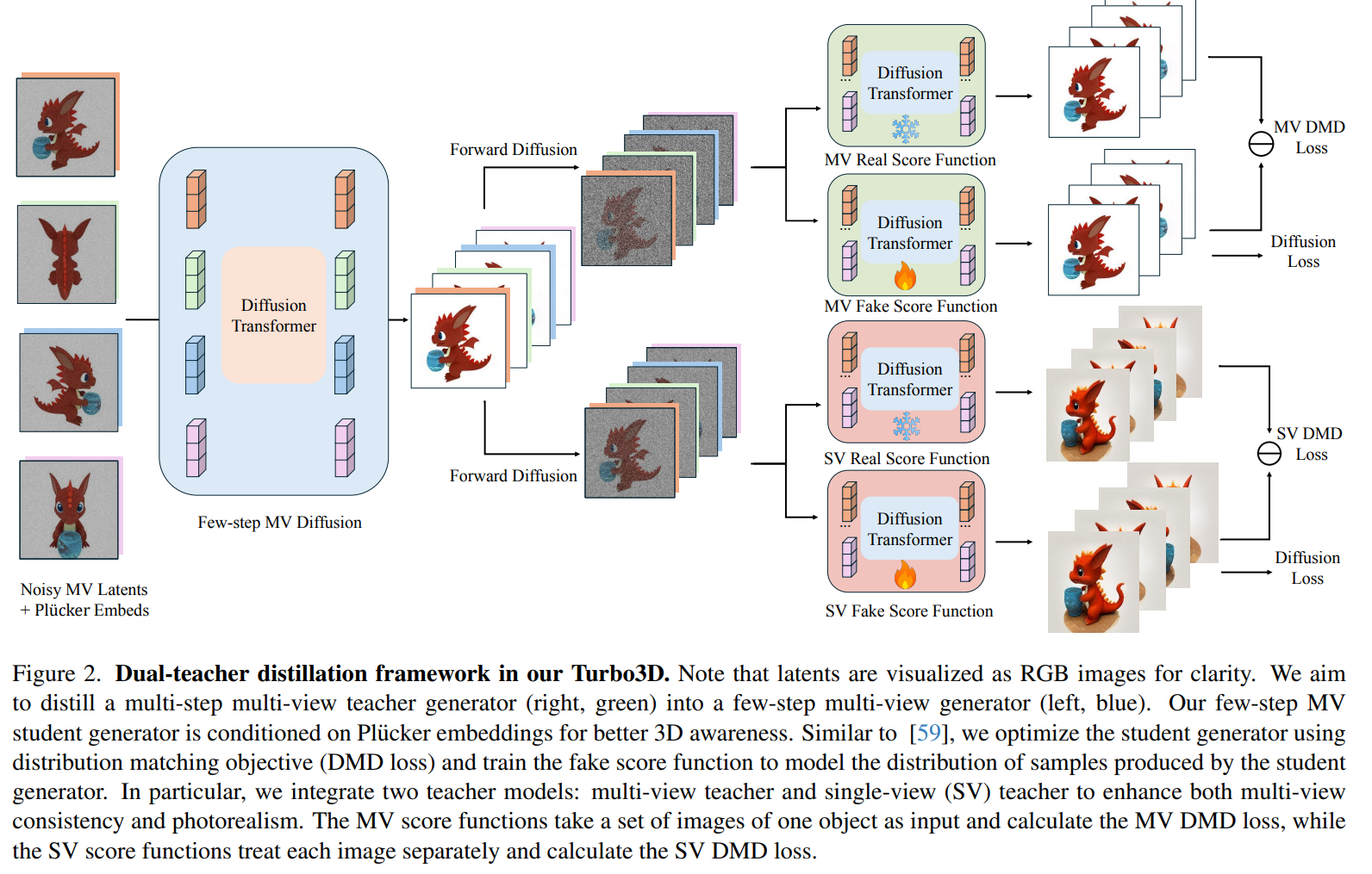
In Fig. 2, the blue block on the left is the few-step MV student diffusion model. The student takes noisy, MV latents, Plücker embeddings as input and generates the latents of multiple views through a Diffusion Transformer.
The paper explains that conditioning the student on Plücker embeddings improves its 3D awareness.
Suppose the four generated views are
\[\{x^1, x^2, x^3, x^4\}\]as shown above. A forward diffusion process at a random timestep $t$ is then applied to obtain
\[\{x_t^1, x_t^2, x_t^3, x_t^4\}\]these noisy views, which are sent through two paths simultaneously, as shown in Fig. 2. The upper path corresponds to Multi-view DMD.
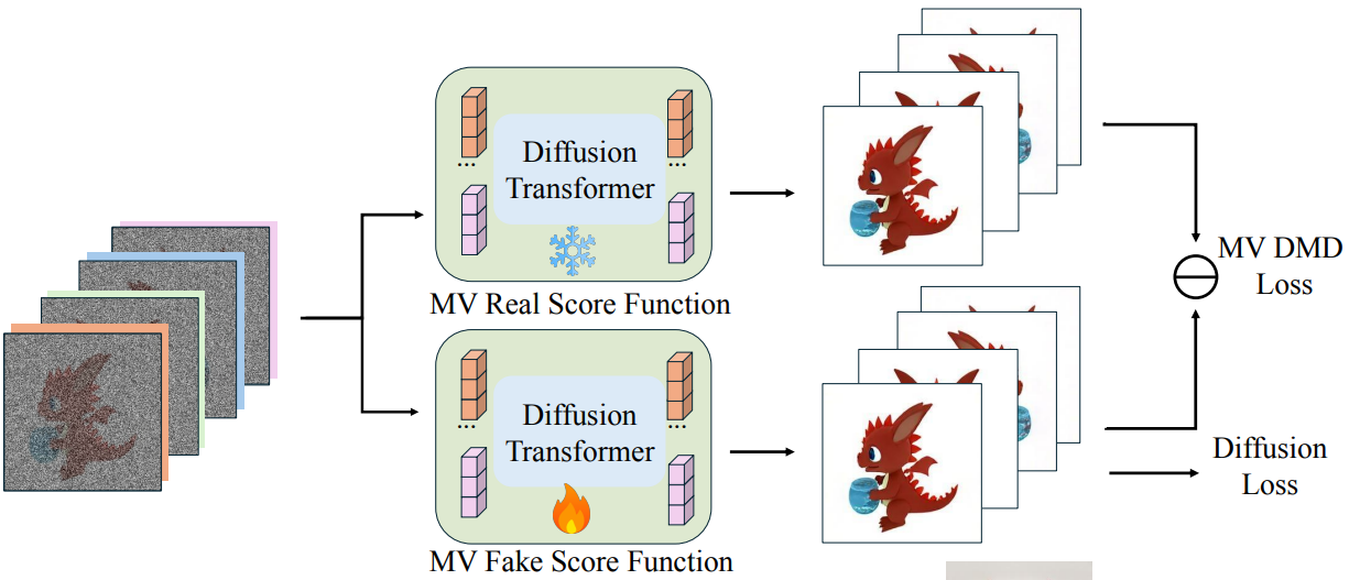
Here, all four views are input together as a set. The DMD loss is computed by comparing the MV teacher’s real score with the fake score of the current student distribution. In other words, the objective is
\[p_{fake} \rightarrow p_{real}^{MV}\]
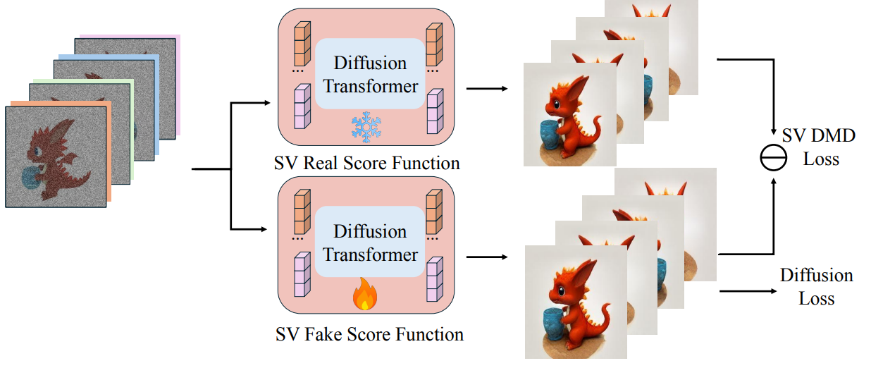
In the lower path, the multi-view sample is split into individual views. Each image is compared with the distribution of the SV teacher. In other words, for each view,
\[p_{fake}(x_t^i) \rightarrow p_{real}^{SV}(x_t^i)\]The paper explains that the MV score function takes the entire image set of one object as input, whereas the SV score function processes each image separately.
The Dual-teacher DMD objective in the paper is defined as follows.
\[L_{\mathrm{DMD}}^{\mathrm{Dual}}(\theta) = D_{\mathrm{KL}} \left( p_{\mathrm{fake}} \left( \{x_t^i\}_{i=1}^{K} \right) \parallel p_{\mathrm{real}}^{\mathrm{MV}} \left( \{x_t^i\}_{i=1}^{K} \right) \right) + \lambda \cdot \frac{1}{K} \sum_{i=1}^{K} D_{\mathrm{KL}} \left( p_{\mathrm{fake}}(x_t^i) \parallel p_{\mathrm{real}}^{\mathrm{SV}}(x_t^i) \right)\]This equation can simply be understood as the sum of two DMD objectives.
The important point in the first term is that the entire set ${x_t^i}_{i=1}^K$ is used. That is,
\[(x_t^1, x_t^2, x_t^3, x_t^4)\]its joint distribution is matched to the MV teacher.
The second term independently performs distribution matching with the SV teacher for each view $i$, and
\[\frac{1}{K} \sum_{i=1}^K\]averages the loss across all views. Turbo3D uses $K=4$ and sets $\lambda = 1$, meaning that the MV and SV teachers are given equal loss weights.
Thus, the loss can be understood intuitively as
\[L_{Dual} = L_{\text{MV-consistency}} + \lambda L_{photorealism}\]as written above.
Latent GS-LRM for MV Reconstruction
The most straightforward approach is to first decode the latents generated by multi-view diffusion into RGB images using a VAE decoder and then feed them into a pixel-space GS-LRM.
However, the authors view VAE decoding itself as unnecessary overhead in this process. In particular, they point out that the Conv2D operations in the VAE decoder can be inefficient in terms of both speed and memory at high resolution.
In other words, since the multi-view generator already produces useful latents, decoding them into RGB only to feed them into another reconstruction model is inefficient.
Turbo3D therefore directly connects the components as follows:
\[\text{MV Latents} \rightarrow \text{Latent GS-LRM} \rightarrow \text{3D Gaussians}\]The paper calls this latent-space reconstructor Latent GS-LRM and trains it to directly take generated MV latents as input and predict 3D Gaussians.
The important point is that training supervision still uses pixel-space novel-view rendering losses.
That is, although Latent GS-LRM takes latents as input, the predicted 3D Gaussians are ultimately rendered from novel views and supervised using L2 and perceptual losses.
Experiments
Setup
The Objaverse dataset is used for training. For multi-view generation, objects are normalized to the range $[-1, 1]^3$, and 16 azimuth views are rendered at an elevation of $20^\circ$. For reconstruction training, 32 random views around each object are used, with a total of 730K objects rendered.
The baselines are Instant3D, LGM, TripoSR, and SV3D. Evaluation uses 400 DreamFusion prompts; for each generated object, 10 random views are rendered to measure the CLIP score, VQA score, and inference time.
The overall training process consists of training the multi-step MV diffusion model, distilling the few-step MV generator, and training Latent GS-LRM. Each training phase uses 32 80GB A100 GPUs.
Evaluation against baselines
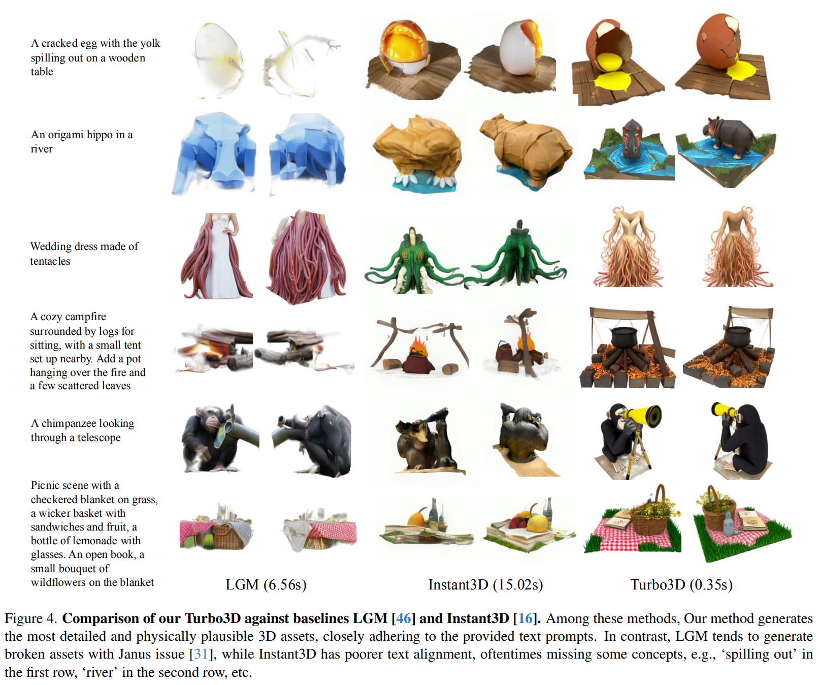
Figure 4 shows that LGM frequently produces simple or broken 3D assets, suffers from the Janus problem, and has poor text alignment. Instant3D is more stable, but can fail to capture detailed concepts or textures in complex prompts. In contrast, the paper claims that Turbo3D produces more detailed, physically plausible results with stronger text alignment even for complex prompts.
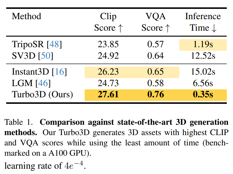
Table 1 shows that Turbo3D achieves higher quality metrics and shorter generation time than the compared methods.
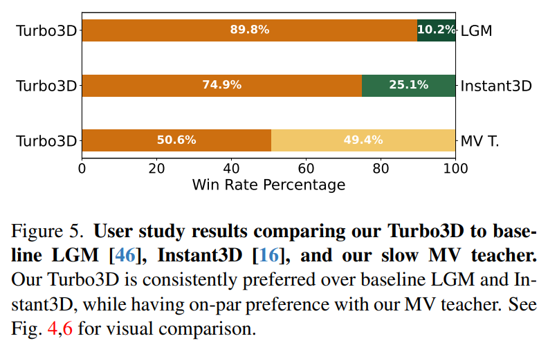
In the user study in Figure 5, 56 users performed 1,120 pairwise comparisons over 80 prompts. Turbo3D was preferred more often than LGM and Instant3D, while showing nearly the same level of preference as its own MV teacher.
Ablation study
This section evaluates the effects of Turbo3D’s two key components: Dual-teacher Distillation and Latent GS-LRM.
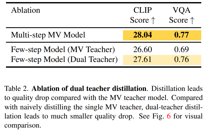
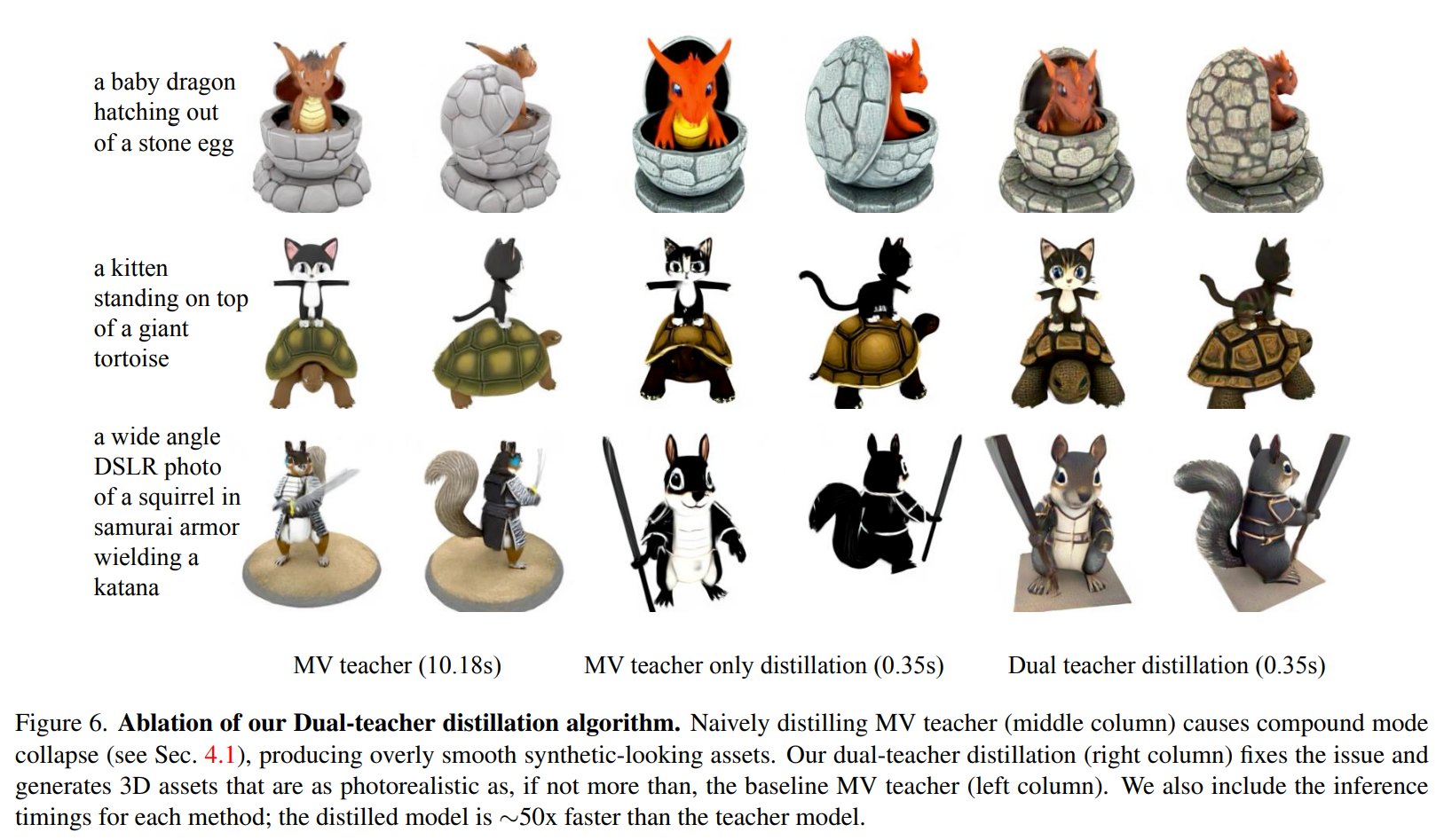
Table 2 and Figure 6 first show that when the multi-step MV teacher is distilled into a few-step model using only the MV teacher, CLIP/VQA scores drop substantially and the outputs become overly smooth and synthetic, exhibiting compounding mode collapse.
In contrast, dual-teacher distillation with the additional SV teacher recovers quality to nearly the level of the MV teacher while retaining the fast few-step inference speed.
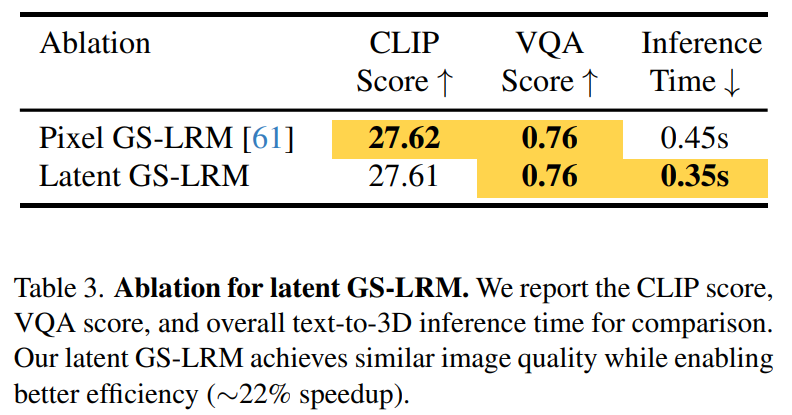
Table 3 compares the original Pixel GS-LRM with Latent GS-LRM, showing that Latent GS-LRM reduces overall inference time by skipping VAE decoding while maintaining nearly identical CLIP/VQA quality.
Contributions
- The paper proposes a system that generates 3DGS assets in under one second.
- It proposes a dual-teacher distillation strategy in which the MV teacher provides multi-view consistency while the SV teacher complements it with photorealism.
- It proposes directly feeding latents into GS-LRM to reconstruct 3D Gaussians.
Limitations & Future work
- The first limitation is the training data. The experiments remain object-centric, and the method has not yet been extended to scene-scale generation.
- The evaluation is relatively weak in terms of 3D metrics that precisely measure the geometry accuracy, surface completeness, and multi-view consistency of actual 3D assets.