[Paper Review, EN] Streaming Autoregressive Video Generation via Diagonal Distillation

Paper Information
Title: Streaming Autoregressive Video Generation via Diagonal Distillation
Authors: Jinxiu Liu, Xuanming Liu, Kangfu Mei, Yandong Wen, Ming-Hsuan Yang, Weiyang Liu
Venue: ICLR 2026
Link: [Paper], [Project], [GitHub]

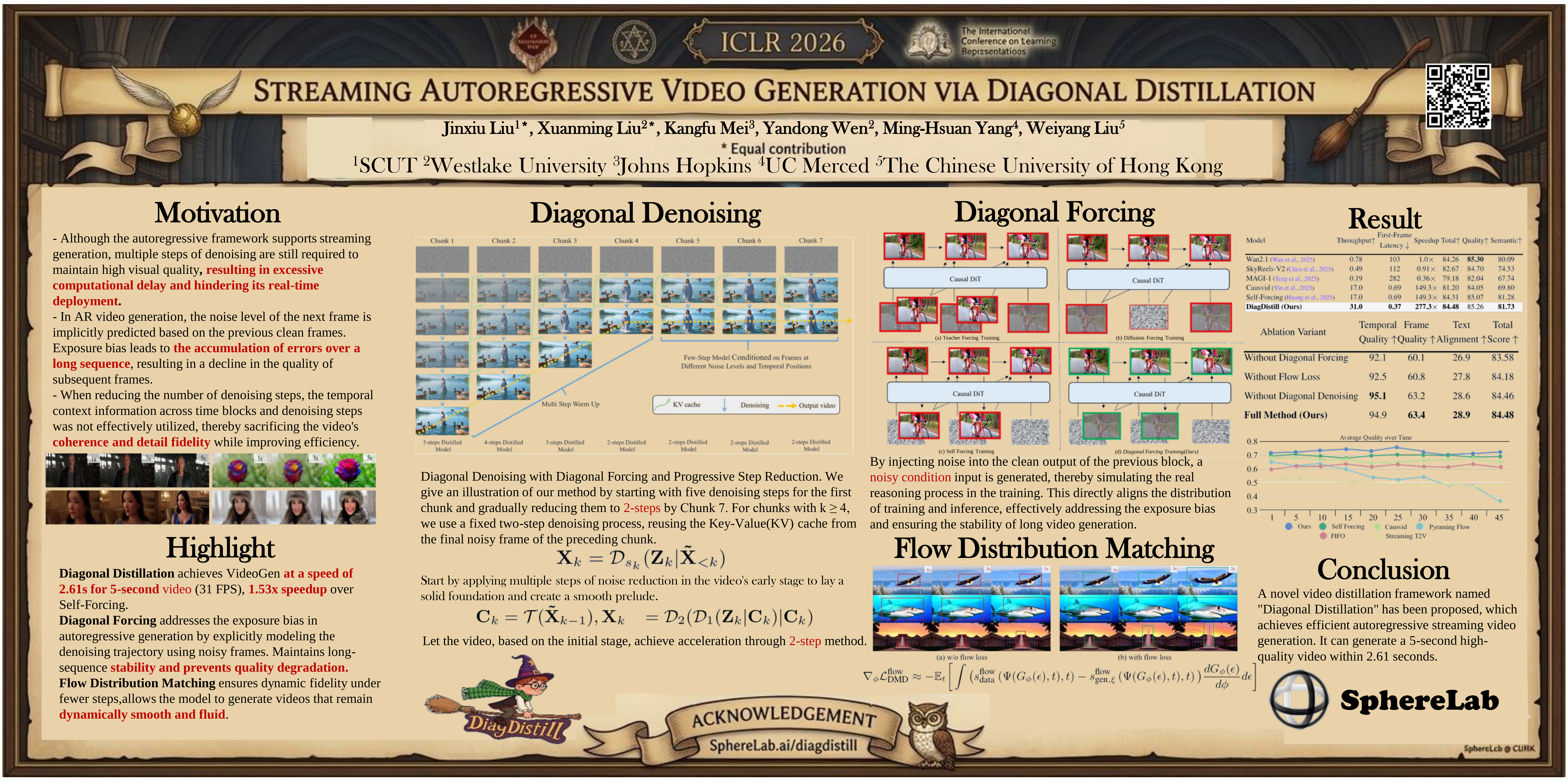
Teaser Image (Poster)

Introduction

Recent advances in diffusion models have enabled video generation to achieve high visual quality. However, most video diffusion models use bidirectional attention, where all frames can attend to one another, and therefore require the entire video to be generated at once. This works well for offline generation, but it is unsuitable for streaming and real-time settings, where future frames are unavailable when generating the current frame. Autoregressive video generation was introduced to address this limitation, providing a structure better suited to streaming by generating videos sequentially at the frame or chunk level. Later, hybrid approaches combining autoregressive modeling and diffusion achieved higher visual quality than conventional GPT-style AR models, but inference latency remained a major issue because each chunk still required multiple denoising steps.

To reduce this computational burden, diffusion distillation has been actively studied. Representative approaches include deterministic methods such as progressive distillation and consistency-based methods, as well as distributional/hybrid methods such as DMD, DMD2, and ADD. However, these methods were mainly developed for image generation, so directly applying them to video often fails to sufficiently capture temporal dependencies and inter-frame consistency. In particular, aggressively reducing the number of denoising steps can weaken motion or degrade temporal coherence, while autoregressive generation can accumulate prediction errors over long sequences because previously generated outputs are repeatedly used as conditions. Recent methods such as CausVid and Self-Forcing have attempted to reduce latency and the train–inference mismatch, but they still require multiple denoising steps and can suffer from quality degradation or oversaturation in long-video generation.

Method & Technical Details

Preliminary

As in many related papers, this paper begins by describing diffusion. When noise is added to the original data $x \sim p_{real}$ according to timestep $t$, we obtain:

\[q_t(x_t | x) \sim \mathcal{N}(\alpha_t x, \sigma_t^2 I)\]

The model takes the noisy sample $x_t$ as input and is trained to predict

\[\mu_{real}(x_t, t)\]

which is close to the original clean sample. The score function is defined as

\[s_{real}(x_t, t) = \nabla_{x_t} log p_{real, t}(x_t) = - \frac{x_t - \alpha_t \mu_{real}(x_t,t)}{\sigma_t^2}\]

Intuitively, as discussed in many previous works, the score is a gradient that tells us “in which direction the current noisy sample should move to approach the real data distribution.”

However, standard diffusion is slow because it requires many denoising steps. DMD, or Distribution Matching Distillation, was introduced to address this. The goal of DMD is to make a few-step student generator match the distribution of a multi-step teacher diffusion model. In other words, the objective is to produce results comparable to those of the teacher model using only a small number of steps.

The paper writes the student as follows:

\[G_{\theta}(z), \; z \sim \mathcal{N}(0, I)\]

This is the notation used for the student generator.

DMD aims to make the distribution $p_{fake}$ generated by the student similar to the real/teacher distribution $p_{real}$. In other words, it minimizes the difference between the two distributions, which the paper formulates using KL divergence as

\[KL(p_{fake,t} || p_{real,t})\]

The objective is to minimize this quantity. The key expression used when updating the student $G_{\theta}$ is

\[s_{real} - s_{fake}\]

This represents how different the score of the teacher/real distribution is from the score of the distribution produced by the student. The student is updated using this difference. For more details on DMD, refer to the Preliminary section of the FlashWorld (ICLR 2026 Oral) paper review page.

The authors then point out a problem. Since DMD was originally developed mainly for image generation,

\[L_{reg} = E_{z,y}d(G_{\theta}(z), y)\]

a loss such as this mainly focuses on matching the quality of each individual frame. In other words, frame 1, frame 2, frame 3, and so on can each be made similar to the teacher, but there is no guarantee that the motion or temporal consistency between Frame 1 $\rightarrow$ Frame 2 $\rightarrow$ … will transition naturally.

The paper describes this as “the regression loss of conventional DMD guarantees per-frame quality but does not explicitly model temporal coherence and long-range dependencies.”

Diagonal Denoising & Diagonal Forcing

This section introduces two core techniques.

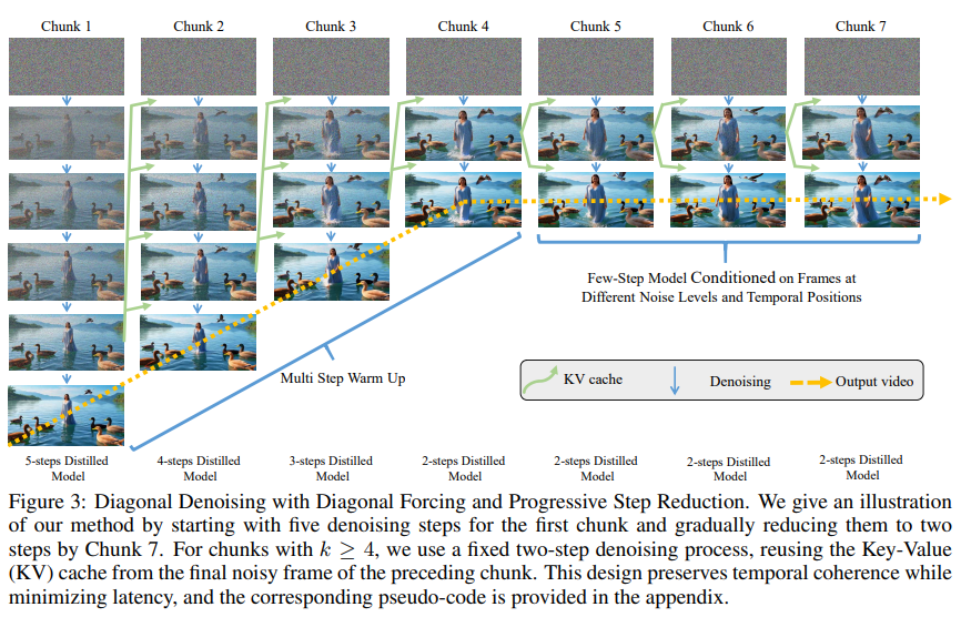
1. Diagonal Denoising: a method that speeds up generation by applying more denoising to earlier chunks and less denoising to later chunks.
2. Diagonal Forcing: a method that passes an appropriately noisy state of the previous chunk through the KV cache/context so that later chunks can still be generated stably with fewer steps.

In conventional autoregressive video diffusion, it is natural to use the same number of denoising steps for every chunk. However, the authors argue that earlier chunks serve as structural priors for later chunks.

That is, if the appearance of the subject, background, and overall structure have already been established in earlier chunks, later chunks are generated using them as context and therefore do not require the same amount of computation from the beginning. Based on this idea, the authors introduce a progressive reduction in the number of denoising steps as the chunks proceed:

\[X_k = D_{s_k} (Z_k | \tilde{X}_{<k}), s_k = 5,4,3\]

Since $Z_k \sim \mathcal{N} (0,I)$, each new chunk itself still starts from Gaussian noise. $D_{s_k}$ is a distilled model that performs $s_k$ denoising steps, and $\tilde{X}_{<k}$ is the noisy context propagated from previous chunks. In other words, later chunks do not start from a less noisy state; instead, they can remove noise with fewer steps because they are given strong temporal context.

From Chunk 4 onward, the process is fixed to 2 steps.

\[C_k = T(\tilde{X}_{k-1})\] \[X_k = D_2(D_1(Z_k | C_k)| C_k)\]

Using information from the previous chunk, the conditioning module $T$ produces conditioning $C_k$, after which only two denoising steps, $D_1$ and $D_2$, are performed.

However, simply reducing the number of steps in the order “5 $\rightarrow$ 4 $\rightarrow$ 3 $\rightarrow$ 2” creates a problem. Suppose that when generating Chunk $k$, the model is conditioned only on the completely clean output of the previous Chunk $k-1$:

\[\text{Chunk} \; k-1 \rightarrow \text{clean output} \rightarrow \text{KV cache} \rightarrow \text{Chunk k}\]

Chunk $k$, however, is currently at a particular noise level in the diffusion/flow denoising process. The model must therefore look at clean context while also implicitly determining which noise level the next chunk should currently be at.

The paper refers to this as the implicit next-noise-level prediction problem and explains that even a small prediction error can accumulate autoregressively. Therefore, rather than using the clean previous chunk directly, the authors deliberately add an appropriate amount of noise before using it (more precisely, a small amount of noise is added to an intermediate latent produced during denoising of the previous chunk, and that representation is stored in the KV cache):

\[\tilde{X}_{k-1} = \sqrt{\alpha_{k-1}} X_{k-1} + \sqrt{1-\alpha_{k-1}} \epsilon, \; \epsilon \sim \mathcal{N}(0, I)\]

$X_{k-1}$ is the clean output of the previous chunk, while $\tilde{X}_{k-1}$ is the same output with controlled noise added. The process then becomes:

\[\text{Chunk} \; X_{k-1} \rightarrow \text{add noise} \rightarrow \text{partially noisy} \; \tilde{X}_{k-1} \rightarrow \text{KV cache} \rightarrow \text{Chunk k}\]

A natural question is why noisy context helps solve this problem. The key is to better align the denoising states of the current chunk and the previous context.

If clean context is used directly, there is a large noise-level mismatch between the Previous Context (Clean) and the Current Chunk (Noisy). In contrast, Diagonal Forcing adds noise to the Previous Context so that its noise level becomes more similar to that of the Current Chunk.

In summary, Diagonal Denoising reduces computation by progressively reducing the number of steps, whereas Diagonal Forcing preserves temporal coherence and long-term stability so that quality does not collapse even when the number of steps is reduced.

Flow Distribution Matching

The authors identify another problem caused by the preceding Diagonal Denoising strategy: motion becomes weaker when generation is compressed to only a few steps. The paper calls this motion attenuation. When the teacher uses enough denoising steps, objects can move substantially and naturally across frames, but when the student is aggressively reduced to around 2 steps, the spatial appearance may still look plausible while the magnitude of motion becomes smaller.

The authors attribute this to the denoising trajectory becoming too short to sufficiently recover temporal dynamics. They therefore argue that DMD alone is insufficient and that the motion distribution itself must also be matched to the teacher:

\[E_{motion} = D_{KL} (p_{teacher}(F(x) | x_t) || p_{student}(F(x) | x_t))\]

Here, $F(x)$ is a motion flow feature extracted from the video. The key idea is “not only to check whether the teacher and student generate similar frames, but also to make the distributions of the motion features produced by the two models similar.”

Conventional DMD aims to match

\[p_{student}(x) \approx p_{teacher}(x)\]

and, in addition, the method also matches

\[p_{student}(F(x)) \approx p_{teacher}(F(x))\]

This can be interpreted as matching both distributions. Flow Distribution Matching is also trained in a DMD-style manner.

\[\nabla_{\phi} L_{DMD}^{flow} = \nabla_{\phi} KL(p_{gen,flow,t} || p_{data,flow,t})\]

In other words, distribution matching in the spatial domain is extended to the motion-feature domain. Therefore,

\[s_{data}^{flow} - s_{gen}^{flow}\]

is used to update the student.

Whereas conventional DMD matches the student image distribution to the teacher image distribution, Flow DMD can be viewed as matching the student motion distribution to the teacher motion distribution.

There is one important point here. The FLOW referred to in this section is not optical flow from an estimator such as RAFT. Instead, motion features are extracted directly from the latent space of the video diffusion model. More specifically,

\[(\text{Latent frame t} - \text{Latent frame t+1}) \rightarrow (X_{t+1} - X_t) \rightarrow \text{Convolution layers} \rightarrow \text{MLP} \rightarrow \text{Motion feature} \; F(x)\]

The method first computes the difference between consecutive latents, applies convolution to extract local motion patterns, and then uses an MLP for feature adaptation. Thus, FLOW here is closer to a learnable motion representation based on latent differences.

The objective of Flow DMD is

\[\nabla_{\phi}L_{DMD}^{flow} = \mathbb{E}[\nabla_{\phi}D_{KL}(p_{gen,flow,t} || p_{data,flow,t})]\]

which encourages the motion-feature distribution produced by the student to approach the real/teacher motion-feature distribution. The flow score is then defined as

\[s^{flow} (x_t, t) = \nabla_{x_t} log p(F(x) | x_t)\]

Unlike the score in standard diffusion, this can be interpreted as a gradient indicating how the current noisy video latent $x_t$ should be changed so that the desired motion feature $F(x)$ becomes more plausible.

\[\nabla_{\phi} L_{\mathrm{DMD}}^{\mathrm{flow}} \approx -\mathbb{E}_{t} \left[ \int \left( s_{\mathrm{data}}^{\mathrm{flow}} \left( \Psi(G_{\phi}(\epsilon), t), t \right) - s_{\mathrm{gen},\phi}^{\mathrm{flow}} \left( \Psi(G_{\phi}(\epsilon), t), t \right) \right) \frac{dG_{\phi}(\epsilon)}{d\phi} \, d\epsilon \right].\]

Ultimately, the generator is trained using $s_{data}^{flow} - s_{gen}^{flow}$, i.e., the difference between the direction preferred by the real/teacher motion distribution and the direction preferred by the student motion distribution.

Here, $\Psi(x,t)$ is a forward noising operation that transforms a video sample $x$ into a noisy state $s_t$ at timestep $t$ (the original DMD formulation appears to use $F$ for the forward noising operation, while this paper uses $F$ for the flow extractor, which is likely why $\Psi$ is used here). A corresponding regression loss is also added to the overall objective.

\[L_{reg}^{flow} = \mathbb{E} [\lVert F(G_{\phi}^{teacher}) - F(G_{\phi}^{student}) \rVert _2^2]\]

Under the same condition, the videos generated by the teacher and student are passed through the teacher/student flow extractor $F(\cdot)$ and aligned. The final loss is therefore

\[L_{\mathrm{Total}} = \lambda_{\mathrm{spatial}} L_{\mathrm{DMD}}^{(\mathrm{grad})} + L_{\mathrm{reg}} + \gamma \left( \lambda_{\mathrm{flow}} L_{\mathrm{DMD}}^{\mathrm{flow},(\mathrm{grad})} + L_{\mathrm{reg}}^{\mathrm{flow}} \right).\]

which gives the overall objective.

Experiments

Implementation Details

Wan2.1-T2V-1.3B is used as the base model, and both ODE initialization and Diagonal Distillation training use text prompts filtered from VidProM and extended with an LLM. Inference is performed on a single NVIDIA H100 GPU using a Tiny VAE and a rolling KV cache with a chunk size of 3 frames. The KV cache retains context from the most recent 4 chunks, keeping the memory footprint fixed at approximately 17.5 GB. Streaming performance is evaluated using both throughput (FPS) and first-frame latency. VBench is used for evaluation: Temporal Quality is the average of subject/background consistency, temporal flickering, motion smoothness, and dynamic degree; Frame Quality is the average of aesthetic/imaging quality; and Text Alignment is the average across multiple semantic dimensions including object, action, color, spatial relation, scene, appearance, and style.

Comparison with state-of-the-art methods

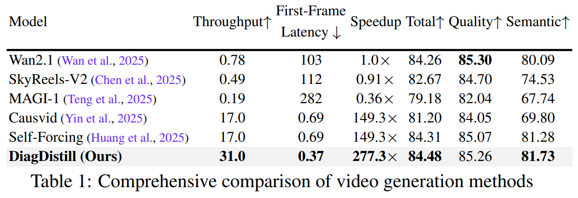
DiagDistill is compared with Wan2.1, SkyReels-V2, MAGI-1, CausVid, and Self-Forcing. On a single H100, DiagDistill achieves 31 FPS with a first-frame latency of 0.37 seconds, corresponding to a 277.3× speedup over Wan2.1, while also providing higher throughput and lower latency than the fast AR baselines CausVid and Self-Forcing. At the same time, it records VBench scores of 84.48 Total, 85.26 Quality, and 81.73 Semantic, maintaining visual quality comparable to the original Wan2.1 while remaining competitive in semantic consistency. Qualitative results also show smoother transitions and fewer distortions than the baselines on complex motions and textures, indicating that the method effectively improves the trade-off between generation speed and quality.

Ablation Studies

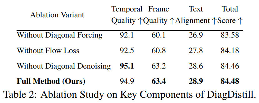
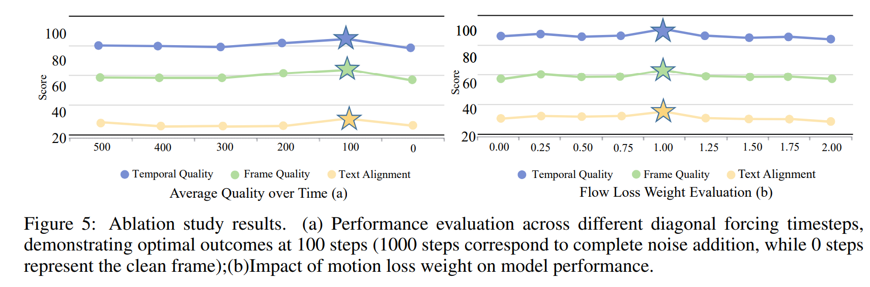
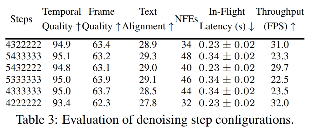
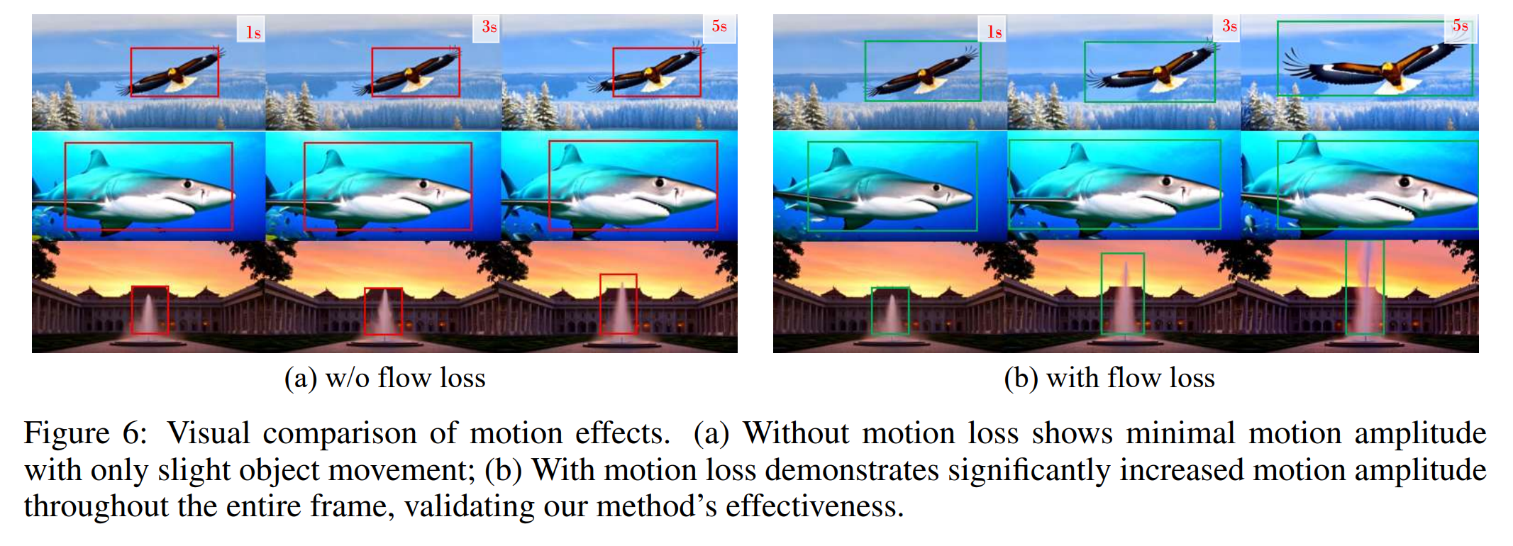
The effects of DiagDistill’s core components and hyperparameters are evaluated by removing or modifying them individually. Table 2 shows that removing Diagonal Forcing causes the largest overall performance drop, while removing Flow Distribution Matching also decreases temporal/frame/text alignment scores. In contrast, removing Diagonal Denoising preserves almost the same quality but increases inference cost, eliminating the speed advantage. Figure 5(a) compares the noise timestep used for Diagonal Forcing and shows that a timestep around 100 performs best; too much noise weakens the structural prior, while too little noise causes over-denoising and oversaturation. Figure 5(b) shows that a flow loss weight of 1.0 provides the best balance among temporal quality, frame quality, and text alignment. Table 3 compares several denoising schedules: 5333333 achieves the highest quality, 4222222 the highest throughput, and 4322222 is ultimately selected as a good balance between quality and speed. Figure 6 additionally visualizes that motion amplitude is substantially reduced without the flow loss, whereas applying the loss preserves more pronounced motion.

Long Video Generation Evaluation

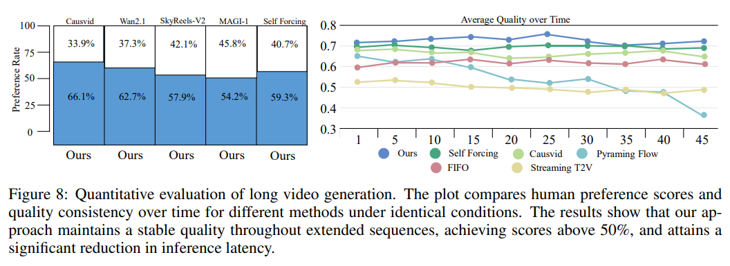
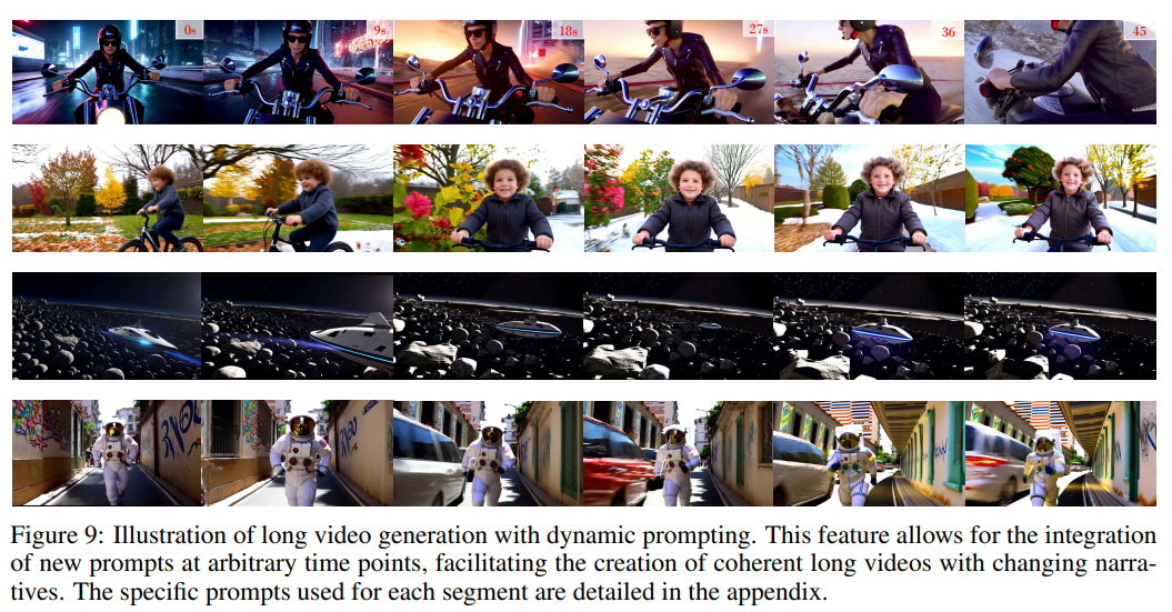
The long-video generation performance of DiagDistill is evaluated. In Figure 8, the perceptual quality of the baselines rapidly decreases over time due to error accumulation, whereas DiagDistill maintains relatively stable quality even over long sequences. A user study with 93 participants on the first 50 prompts from MovieGenBench also shows a higher preference for DiagDistill than the baselines in overall visual quality, text faithfulness, and long-term consistency. This is consistent with the qualitative comparison in Figure 7, where CausVid and Self-Forcing exhibit saturation distortion and quality degradation during long-duration generation. Figure 9 further demonstrates dynamic prompting, which allows a new prompt to be introduced at an arbitrary point during generation, enabling the continuous generation of long narrative videos in which scenes or actions change over time.

Contributions

• Instead of using the same number of denoising steps for every video chunk, the method allocates more steps to early chunks and progressively fewer steps to later chunks, reducing computation while leveraging temporal context.
• The denoising trajectory and partially noised representation of the previous chunk are propagated to the next chunk as a contextual prior/KV cache, reducing the mismatch between training and inference and mitigating error accumulation in long-video generation.
• To compensate for motion degradation and reduced motion amplitude in few-step denoising, the method adds a temporal distillation objective that aligns the motion distributions of the teacher and student.

Limitations & Future works

• Looking at the output videos on the GitHub page, there are cases where a vehicle moving forward suddenly transitions into a scene where it moves backward. This suggests that the method does not always guarantee outputs that are physically consistent or consistent with the temporal flow.
• The reported real-time performance relies on optimizations such as the H100 GPU, Tiny VAE, and rolling KV cache, so it does not imply that the same 31 FPS can be guaranteed across all hardware or base models.