[Paper Review, EN] Lyra 2.0: Explorable Generative 3D Worlds

Paper Information
Title: Lyra 2.0: Explorable Generative 3D Worlds
Authors: Sherwin Bahmani, Tianchang Shen, Jiawei Ren, Jiahui Huang, Yifeng Jiang, Haithem Turki, Andrea Tagliasacchi, David B. Lindell, Zan Gojcic, Sanja Fidler, Huan Ling, Jun Gao, Xuanchi Ren
Venue: SIGGRAPH Asia 2026
Link: [Paper], [Project], [Github]

Teaser Image

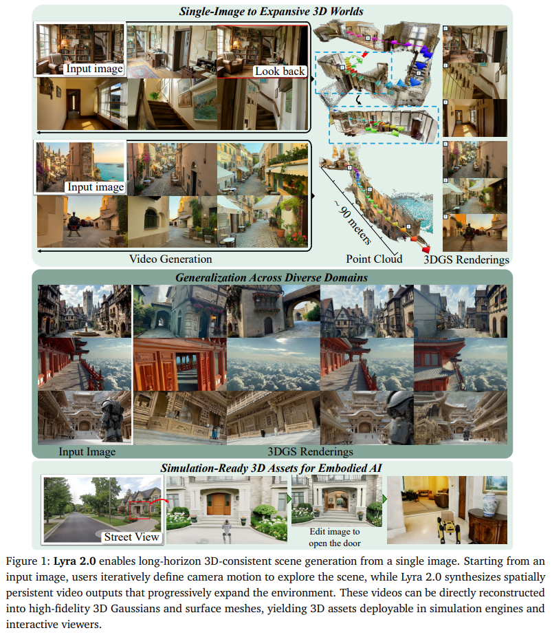
Introduction

Lyra 2.0 is a framework that generates long-horizon, explorable, 3D-consistent worlds from a single image and a user-specified camera trajectory. Existing camera-conditioned video generation methods show high quality and good camera control over short sequences, but two problems arise during long autoregressive generation:

1. Spatial forgetting, where the model fails to correctly remember the structure of a region when revisiting it after that region has fallen outside the temporal context.
2. Temporal drifting, where accumulated small errors during generation gradually degrade color and geometry.

To address these problems, previous works have injected camera information using camera poses, Plücker rays, or depth warping, and have attempted to maintain long-term consistency through past-frame retrieval, global 3D memory, latent/KV caches, or FramePack-based history compression. However, methods that directly use a global 3D representation for conditioning can amplify errors as inaccurate depth estimates or generation artifacts accumulate, while simply adding history frames makes it difficult to establish accurate geometric correspondence under large viewpoint changes.

To address these limitations, Lyra 2.0 does not fuse the 3D geometry of each frame into a single global scene, but instead maintains per-frame 3D memory. The geometry is used only for information routing, specifically for relevant history-frame retrieval and dense correspondence computation, rather than for directly generating appearance. In addition, self-augmentation uses the model’s own imperfect generations as history conditions to improve robustness to temporal drifting. The generated videos are then converted into 3D Gaussians and surface meshes, enabling broader and more persistent 3D scene exploration than previous generative reconstruction approaches.

Method & Technical Details

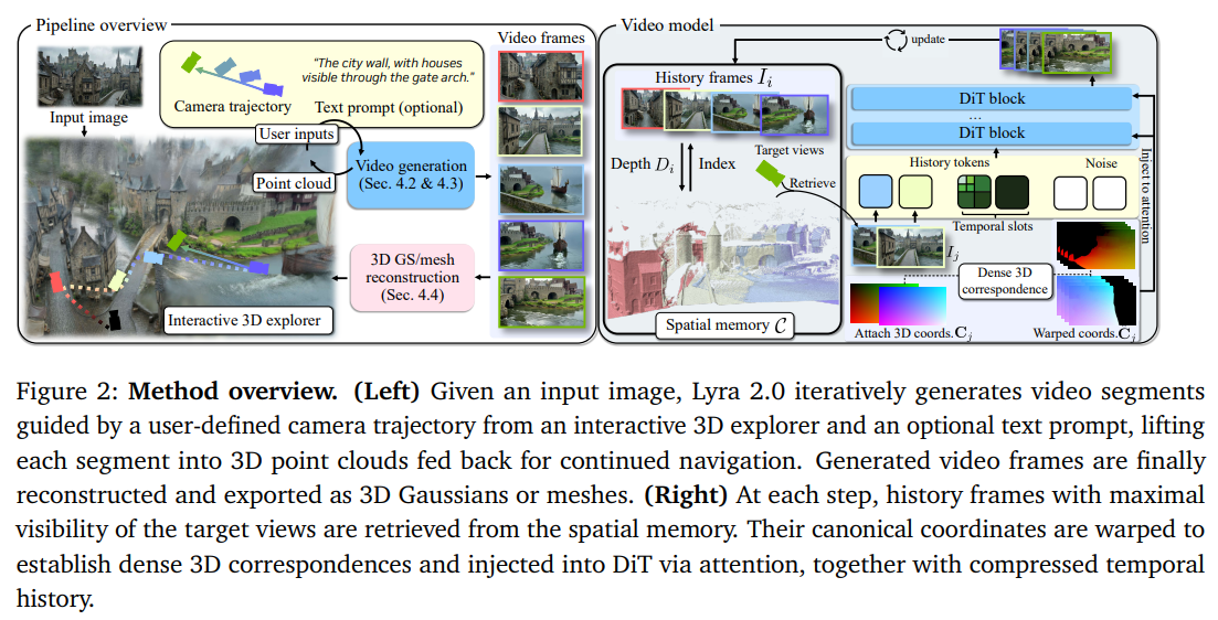
First, let us examine the overall pipeline.

Lyra 2.0 takes three main inputs:

1. single image $I_0$
2. the full camera trajectory specified by the user ${(T_i, K_i)}_{i=0}^{T-1}$
3. and, optionally, a text prompt

However, rather than generating a video for the entire trajectory at once, it repeats an autoregressive retrieve-generate-update loop(this seems to extend the future-work direction mentioned in the original Lyra paper).

That is, given the target viewpoint for the next segment to be generated, it first retrieves the past frames that are most relevant to that viewpoint in 3D, uses that information to generate the next video segment, and then adds the newly generated frames and geometry back into memory.

More specifically:

• Retrieve: Select past frames from spatial memory that have high 3D overlap with the target view to be generated
• Generate: Generate the next video chunk by conditioning jointly on the selected spatial history and recent temporal history
• Update: Estimate the depth and 3D point cloud of the newly generated frames and add them to spatial memory

As generation continues, the memory keeps growing. Importantly, this memory is not merely a temporal context that stores only the “previous few frames”; it is a spatial memory that can retrieve regions seen hundreds of frames earlier based on their 3D locations.

Thus, in the left block of the overview figure above,

\[\text{Input image} \rightarrow \text{camera trajectory} \rightarrow \text{video generation} \rightarrow \text{point cloud update}\]

is satisfied, and the final generated video frames are used to perform 3DGS or mesh reconstruction.

In the Introduction, we identified two major problems: forgetting and drifting. The paper introduces two core modules to address them, which are discussed in detail below.

Anti-Forgetting for 3D-Persistent Video Generation

This technique addresses the following question.

When the camera looks back at a place seen a long time ago, how can the model remember that space and generate it with the same appearance as before?

To solve this problem, Lyra 2.0 does not use 3D geometry as a condition that directly produces appearance. Instead, it uses geometry only for information routing, telling the model “which past frames should be retrieved” and “which locations in those frames correspond to which locations in the current view.”

The overall anti-forgetting pipeline can be summarized as follows:

\[\boxed{ \text{Build 3D cache} \rightarrow \text{Geometry-Aware Retrieval} \rightarrow \text{Spatial Memory Injection} }\]

In other words,

1. store the 3D information of all frames generated so far,
2. retrieve past frames relevant to the target view to be generated, and
3. construct 3D correspondences between those frames and the target view and feed them into the video model.

Building the 3D Cache

First, Lyra 2.0 updates the 3D cache $\mathcal{C}$ whenever new video frames are generated.

For each frame $I_i$, the known or estimated quantities are

\[I_i, D_i, T_i, K_i\]

which correspond to the RGB frame, estimated depth, camera extrinsic, and camera intrinsic, respectively.

The depth $D_i$ is then used to construct a 3D point cloud. The paper represents it as

\[P_i \in \mathbb{R}^{(\frac{H}{d}) \times \frac{W}{d} \times 3}\]

This means that the full-resolution depth is not converted directly into a point cloud. Instead, it is subsampled by a factor of $d$ and unprojected into world coordinates. The appendix uses $d=8$.

However, Lyra 2.0 does not merge these into a single global point cloud.

One might naturally consider merging the point clouds from all frames,

\[P_0, P_1, ...\]

into a single $P_{global}$, but Lyra 2.0 does not do so.

Instead, it stores the geometry of each frame,

\[P_0, P_1, ...\]

independently, because the depth is not ground truth but is estimated from generated images. Even for the same object, the depth estimator may predict different values in different frames. Continuously fusing them into a single global point cloud would accumulate depth errors and cross-view misalignment, eventually corrupting the global geometry.

Therefore, Lyra 2.0 maintains per-frame 3D geometry.

Geometry-Aware Retrieval

Now suppose we need to generate a frame from a new target viewpoint.

Let the target camera be

\[(T^*, K^*)\]

The problem is that there may be hundreds of history frames, and they cannot all be fed into the DiT. Therefore, only the $N_s$ history frames most relevant to the current target view must be selected. The paper uses $N_s=5$.

We therefore need a way to measure how relevant each frame is to the target view.

Each history frame’s point cloud $P_i$ is projected into the target camera $(T^, K^)$. That is,

\[P_i \xrightarrow{T^*, K^*} \text{target image plane}\]

This allows us to determine where 3D points observed in past frames would appear in the current target camera and how many points from a particular past frame fall within the current target image region.

However, simply counting projected points is insufficient because points that are occluded behind other surfaces can still project onto the target image. Therefore, when multiple points are projected to the same target pixel,

\[d_{min}(u,v)\]

the nearest projected depth is computed. If the depth of a point from history frame $i$ is $d_i$,

\[|d_i - d_{min}| < \delta\]

the point is considered visible only when this condition holds. The appendix uses $\delta=0.1$ in normalized depth units. Thus, occluded points behind the visible surface are excluded from the visibility computation.

The number of points judged to be visible is then counted to obtain

\[\phi(i)\]

which can be interpreted as the number of points in $P_i$ visible from the current target view. For example, if $\phi(20)=5000, \; \phi(300)=120$, frame 20 is considered much more relevant. In other words, the method considers spatial overlap rather than temporal proximity.

The retrieval strategy differs slightly between training and inference. During training, frames are sampled in proportion to their visibility scores. Instead of always selecting only the best frames, frames with higher visibility are selected with higher probability. This makes the model robust to variations in retrieval results.

At inference, the method uses greedy coverage rather than simply selecting the top-scoring frames, because the top frames could all have been captured from nearly the same viewpoint. Therefore, during inference it:

1. selects the frame that covers the largest number of target pixels not yet covered
2. marks that region as covered
3. selects the frame that covers the largest portion of the remaining uncovered region
4. repeats this process

until $N_s$ frames have been selected. This increases the likelihood of selecting history frames from diverse viewpoints.

Injecting Spatial Memory into the Video model

We have now determined which history frames to use. Let the selected history frames be

\[\{I_j\}_{j=0}^{N_s - 1}\]

These frames are converted into spatial slots, with each frame encoded independently by the VAE.

The important point is that they are encoded independently as image tokens without temporal compression, unlike ordinary video. This is because the selected history frames are not five temporally consecutive frames. Therefore, each frame is independently encoded as a single image.

As a result, spatial downsampling is applied through VAE compression.

\[H \times W \rightarrow \frac{H}{8} \times \frac{W}{8}\]

FramePack’s spatial compression (patchification/subsampling) is then applied. In other words, the already constructed latents/tokens are further spatially subsampled to reduce the number of tokens.

\[f_{nkm}\]

This notation means that $n$ frames are compressed with a spatial subsampling factor of $m$. For example, suppose five history frames are retrieved:

\[I_{20}, I_{105}, I_{230}, I_{450}, I_{700}\]

Each of these five frames is first passed independently through the VAE. Since using full-resolution tokens for all five would be expensive, four of them are spatially compressed with $k=2$, while one uses $k=1$, meaning it retains the resolution after VAE encoding.

This is written as $f_{4k2}, f_{1k1}$. Simply put,

among the five retrieved history frames, four are provided as low-resolution tokens and one as high-resolution tokens.

That is what the notation means.

However, if only history images are provided, it is difficult for the model to know that a specific pixel in a history image and a specific pixel in the target image correspond to the same 3D point.

Therefore, Dense 3D Correspondence is added.

For each retrieved frame $j$, a canonical coordinate map

\[C_j \in [-1,1]^{3 \times H \times W}\]

is constructed. Each pixel is represented as

\[C_j(u,v) = (u,v,2\frac{j}{N_s}-1)\]

The first two channels, $u,v$, indicate where the pixel was located in the source image. The third value serves as a frame identity that distinguishes which spatial slot/frame the pixel came from.

In other words,

\[(u,v,j)\]

can be regarded as being encoded into three coordinate channels.

The source-frame depth $D_{s_j}$ and camera poses are then used to forward-warp $C_j$ into the target camera:

\[\hat{C_j} = FwdWarp(C_j, D_{s_j}, T_{s_j}, T^*, K_{s_j}, K^*)\]

This corresponds to

\[\text{source pixel} \rightarrow \text{3D world} \rightarrow \text{target pixel}\]

Thus, if $(u_s, v_s, j)$ appears at a certain location in the target image, it means that “this target pixel corresponds to location $(u_s,v_s)$ in the $j$-th image of spatial memory.”

In addition to the three canonical-coordinate channels, depth is also warped to construct, for each source frame (the five selected history frames),

\[[\hat{C_j}; \hat{D_f}]\]

a 4-channel correspondence map containing (u,v,frame ID, depth). Thus, this is not merely a 2D correspondence, but a 3D-aware dense correspondence.

This correspondence map

\[[\hat{C_j}; \hat{D_f}]\]

is converted into an embedding through positional encoding and an MLP. Specifically,

\[[\hat{C_j}; \hat{D_f}] \rightarrow \text{pixel shuffling} \rightarrow \text{sinusoidal positional encoding} \rightarrow \text{linear projection}\]

is used to match the token dimension. This embedding is then added to the transformer’s Q and K.

\[q = W_Q(x+p_{corr}) \\ k = W_K(x+p_{corr})\]

The value is left unchanged because the purpose is to tell the attention mechanism which tokens should attend to which spatial-memory tokens.

In other words, Q and K are modified to guide attention matching, while V, which carries the actual appearance information, retains the features of the pretrained video model.

The discussion above was lengthy, so to summarize, the input to the DiT can ultimately be viewed as

\[X = [X_{anchor}, X_{spatial}, X_{temporal}, X_{generate}]\]

This is the overall structure.

Here, Anchor denotes the initially provided image $I_0$; Spatial tokens are the VAE features of five history frames selected through 3D retrieval; Temporal tokens are compressed features of recent generation history produced by FramePack; and Generate tokens are the noisy latents of the target video chunk currently being generated.

The correspondence map is not concatenated as part of the input above. Instead, after processing, it becomes an embedding that modulates attention and is injected into the DiT’s Q and K.

Anti-Drifting for Long-Horizon video Generation

During training, the model typically receives clean ground-truth history frames as conditioning. At inference, however, ground truth is unavailable, so it must condition on frames generated by the model itself. That is,

\[\hat{x}^{hist} \rightarrow \text{generate next chunk}\]

If the previous generation contains even small amounts of blur, color shift, or geometry error, the next chunk is generated from that imperfect history, and the following chunk is again generated from the resulting output. Errors can therefore accumulate over time.

The paper refers to this as observation bias.

Lyra 2.0 already uses FramePack, which aggressively compresses distant history while preserving recent history at finer granularity, allowing a longer temporal context within a limited token budget. It also keeps the initial image as an anchor, which helps prevent the generation from drifting too far from $I_0$.

However, FramePack is designed to expose the model to a longer history, not to train it to produce correct outputs from imperfect history. Therefore, the train-test gap still remains.

The paper discusses Self-Forcing as a related idea. It reduces the train-test gap by conditioning the model on its own predictions during training as well. However, to construct training-time histories that resemble actual inference, each history segment would need to be fully generated. This can require multiple denoising steps over the history for every training sample, making it prohibitively expensive.

The authors therefore propose Self-Augmentation Training. In simple terms,

during training, expose the model to a “slightly degraded history” as it would see at inference, and train it to generate the next chunk correctly even under that condition.

First, a training sample is divided into

\[x^{hist}, x^{cur}\]

the previous history segment and the current target chunk to be generated. Both are first VAE-encoded using ground-truth frames.

\[z_0^{hist} = \mathcal{E}(x^{hist})\]

Because the current chunk is encoded by a causal VAE, it uses the history cache as conditioning to obtain

\[z_0^{hist} = \mathcal{E}(x^{cur} | x^{hist})\]

the resulting latent.

Next, self-augmentation is applied to the history with probability $p_{aug}=0.7$. Here, $p_{aug}$ is the probability of deciding whether or not to apply self-augmentation to a given training sample. Then,

\[t \sim \mathcal{u}(0, 0.5)\]

a value $t$ is sampled from a uniform distribution between 0 and 0.5. This can be interpreted as the noise strength that determines how severely the history is corrupted. After sampling $t$,

\[z_t^{hist} = (1-t)z_0^{hist} + t \epsilon\]

noise is added to the history latent, producing a noisy history. However, this noisy history is not used directly as conditioning; instead, the video model performs exactly one denoising step.

\[\tilde{z}_0^{hist} = z_t^{hist} - t v_{\theta}(z_t^{hist}, t, c)\]

This produces

\[\tilde{z}_0^{hist}\]

a slightly imperfect pseudo-history $\tilde{z}_0^{hist}$, which is then used as conditioning instead of the clean history.

The important point is that the target remains clean. In other words, the supervision uses

\[z_0^{cur}\]

as the clean target.

The authors argue that this makes the model robust to error propagation caused by its own bias or reconstruction errors.

3D Reconstruction

The long 3D-consistent video generated above must now be converted into actual 3DGS and mesh representations.

The authors use Depth Anything V3 to predict per-pixel 3DGS attributes from the input frames in a feed-forward manner. However, the original DAv3 predicts one Gaussian per pixel, resulting in too many Gaussians for high-resolution videos. To address this, they modify the Gaussian DPT head so that its output feature map is downsampled by a factor of $K \times K$. This reduces the number of Gaussians to $\frac{1}{k^2}$ of the original count. The actual setting is $k=2$.

If needed, the 3DGS is further converted into a surface mesh using an OpenVDB-based hierarchical sparse grid. Although 3DGS, as a set of Gaussian primitives, is well suited for rendering, triangle meshes can be more convenient for representing object surfaces and collisions in simulators such as Isaac Sim. Therefore, depth is rendered from the Gaussians and used to reconstruct the surface.

To reconstruct the surface, a normal vector $n$ is required to describe the surface orientation of each 3D point after unprojection. The normals are computed from the depth gradients. Thus,

\[(p,n)\]

forms a single oriented point, and the resulting set of points is called an oriented point cloud. The method additionally uses a Signed Distance Field, which represents both the distance to the nearest surface and, through its sign, whether a location lies outside or inside the surface.

On the surface, $S(x)=0$; outside the surface, $S(x)>0$; and inside, $S(x)<0$. Marching Cubes extracts a mesh from the zero level set of the SDF, so locations where $S(x)=0$ correspond to the surface. It traverses the voxel grid, identifies where the SDF changes sign from positive to negative within each voxel, and constructs a triangle mesh.

Distilled Model for Accelerated Inference

The original Lyra 2.0 model performs 35-step denoising at inference. The authors use this model as the teacher and train a 4-step student model using DMD.

CFG is distilled as well. Ordinarily, CFG requires separate conditional and unconditional predictions at inference, typically resulting in two forward passes per denoising step. Lyra 2.0 distills this guidance effect directly into the student, allowing single-pass inference without separate conditional and unconditional forward passes.

Self-augmentation is also retained during distillation.

According to the appendix, an 80-frame step takes 15 seconds with the distilled model, compared with 194 seconds for the original full model, corresponding to an approximately 13× speedup.

Experiments

Training Details

Lyra 2.0 is trained on the DL3DV dataset. Camera poses are estimated using ViPE, depth using Depth Anything V3, and captions using Qwen3-VL-8B-Instruct. During training, 30% of samples use single-image-conditioned I2V training, while the remaining 70% use autoregressive chunk-based training with previous frames as history.

Long Video Generation & 3D Scene Generation

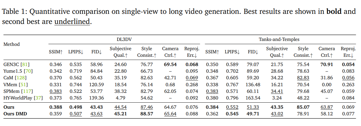
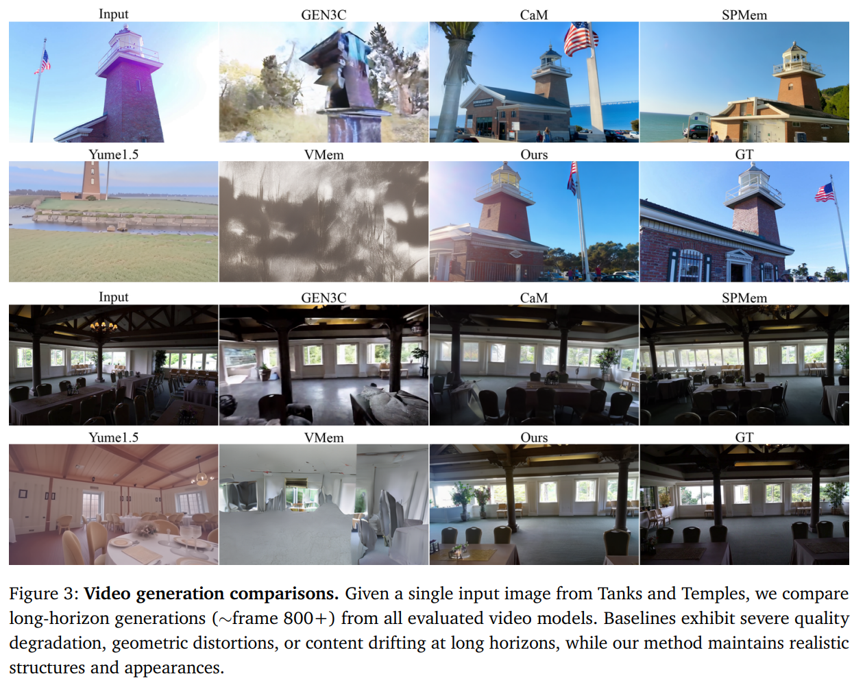
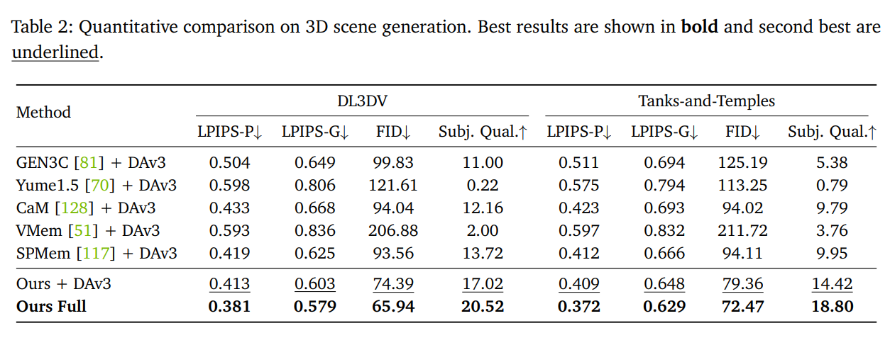
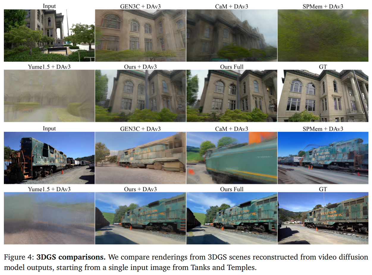
The baselines are GEN3C, Yume-1.5, CaM, VMem, SPMem, and HY-WorldPlay, evaluated on DL3DV-Evaluation and Tanks and Temples. The main metrics are SSIM, LPIPS, FID, Subjective Quality, Style Consistency, Camera Controllability, and Reprojection Error.

Lyra 2.0 achieves the best performance on most metrics and, in particular, maintains strong visual quality, camera control, and long-range consistency even over long generations. The DMD version reduces the number of denoising steps from 35 to 4 while maintaining comparable quality, although camera controllability decreases moderately.

The generated videos are reconstructed into 3DGS using DAv3 and evaluated with LPIPS-P, LPIPS-G, FID, and Subjective Quality. In particular, Ours Full, which uses DAv3 fine-tuned on Lyra-generated videos, achieves the best performance, showing that the improved 3D consistency of the generated videos translates into better reconstruction quality.

Ablation Study

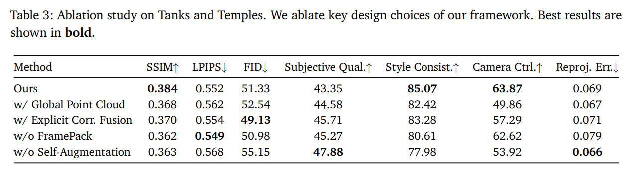
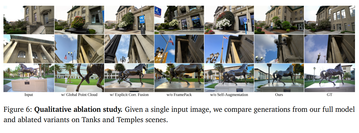
The main ablations are as follows.

• Global Point Cloud: camera control and style consistency decrease due to accumulated depth errors
• Explicit Correspondence Fusion: performs worse than learned aggregation
• w/o FramePack: temporal drifting and reprojection error increase
• w/o Self-Augmentation: long-range style consistency and camera controllability decrease

These results confirm that per-frame spatial memory, learned correspondence aggregation, FramePack, and self-augmentation are all important.

Applications

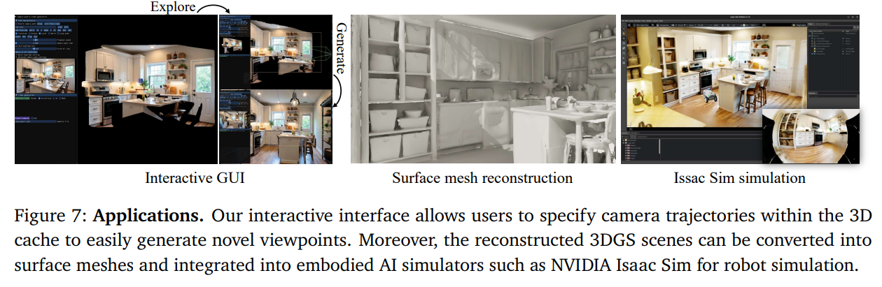
Lyra 2.0 demonstrates applications including scene exploration through an interactive GUI, in-the-wild single-image 3D scene generation, and embodied AI simulation by importing the generated meshes into NVIDIA Isaac Sim.

Contributions

• Maintains spatial consistency in long-horizon video generation through an anti-forgetting mechanism based on per-frame 3D spatial memory and dense correspondence.
• Mitigates error propagation and temporal drifting in autoregressive generation through self-augmentation training.
• Converts the generated long videos through feed-forward 3DGS reconstruction to create large-scale, explorable 3D worlds and further provides simulation-ready meshes.

Limitations & Future works

• Lyra 2.0 currently focuses only on static environments and does not explicitly model dynamic scenes. Extending the framework to dynamic scenes remains an important direction for future work.
• Exposure variation in DL3DV may also appear in the generated videos, and such photometric inconsistencies can cause artifacts in feed-forward 3DGS reconstruction.
• Future work could improve the network’s photometric stability or use photometrically consistent synthetic datasets from game engines to achieve more stable 3D scene generation.