[Paper Review, EN] Layered 4D-Rotor Gaussian Splatting: A Compressed Representation for Long Dynamic Scenes

Paper Information
Title: Layered 4D-Rotor Gaussian Splatting: A Compressed Representation for Long Dynamic Scenes
Authors: Hanjie Xu, Yuanxing Duan, Qiyu Dai, Ge Li, Baoquan Chen, He Wang
Venue: CVPR 2026
Link: [Paper], [Project]

Teaser Image

Introduction

The most challenging aspect of representing Dynamic Environments is modeling complex spatio-temporal deformations and diverse motion patterns. In particular, modeling them across changes in time and viewpoints is even more difficult.

In other words, dynamic novel view synthesis remains under-explored. Existing NeRF-based NVS approaches suffer from slow volume rendering, making real-time or long-duration applications difficult, and 3DGS emerged to address these limitations. Nevertheless, although existing 3DGS methods perform well on short videos, they suffer from high GPU VRAM usage and storage requirements for long videos because the number of Gaussians increases rapidly.

For long videos, a method called Temporal Gaussian Hierarchy (TGH) has studied 4D Gaussians, but it still cannot satisfy low-bandwidth requirements for environments such as mobile platforms.

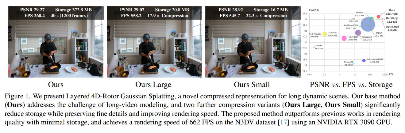
Therefore, this paper introduces a new framework called Layered 4D-Rotor Gaussian Splatting (L4DRotorGS), which enables high-fidelity reconstruction and real-time rendering while reducing storage costs.

Method & Technical Details

Preliminary of 4D-Rotor Gaussian Splatting

The authors include this section because understanding the SIGGRAPH 2024 paper “4D-Rotor Gaussian Splatting: Toward Efficient Novel View Synthesis for Dynamic Scenes” is required as preliminary knowledge.

To first summarize the core idea of the 4DRGS paper,

4D-Rotor GS represents each Gaussian not as a simple 3D ellipsoid, but as a 4D ellipsoid in x, y, z, t space, and obtains the 3D Gaussian at a desired time t by slicing this 4D ellipsoid.

First, standard 3D Gaussian Splatting has

\[\mu = \begin{bmatrix} \mu_x \\ \mu_y \\ \mu_z \end{bmatrix}\]

as its center and

\[\Sigma \in \mathbb{R}^{3 \times 3}\]

as its covariance, and

\[G(x) = \text{exp}(-\frac{1}{2}(x-\mu)^T \Sigma^{-1} (x-\mu))\]

is represented as above. In addition, rather than optimizing the covariance directly, it is decomposed into scale and rotation.

Typically,

\[\Sigma = RSS^TR^T\]

and

\[S = diag(s_x, s_y, s_z)\]

This gives the scale matrix used in the covariance decomposition.

Adding opacity and SH coefficients gives the standard 3DGS primitive that we are familiar with.

In a dynamic scene, a Gaussian must represent not only where it exists in (x, y, z), but also how it exists over t. Therefore, 4DRotorGS lifts the Gaussian itself into (x, y, z, t) space. In other words, it represents a 3D Gaussian as a 4D Gaussian.

This can be understood as follows.

Instead of constructing a separate 3D scene for every time step, slicing a single XYZT Gaussian with a temporal plane yields the 3D Gaussian at each time.

If the center of a 3D Gaussian is \((\mu_x, \mu_y, \mu_z)\), then in 4D it becomes

\[\mu_{4D} = (\mu_x, \mu_y, \mu_z, \mu_t)\]

Here, \(\mu_t\) should be understood not as a frame index, but as “the time at which this Gaussian is centered along the temporal axis.” In other words, it is strongest when \(t=\mu_t\) and becomes weaker as it moves farther away in time. In the original paper, the sliced Gaussian is multiplied by

\[e^{-\frac{1}{2} \lambda (t-\mu_t)^2}\]

which reaches its maximum at \(\mu_t\) and vanishes as the time moves farther away.

Then the covariance also becomes

\[\Sigma_{4D} = R_{4D}S_{4D}S_{4D}^TR_{4D}^T\in \mathbb{R}^{4 \times 4}\]

This gives the corresponding 4D covariance.

Therefore,

\[G_{4D}(x) = \text{exp} (-\frac{1}{2} (x-\mu_{4D})^T \Sigma_{4D}^{-1} (x-\mu_{4D}))\]

where \(x = (x,y,z,t)^T\).

Intuitively, a tilted 4D Gaussian produces motion. For example, suppose a Gaussian is tilted in the x-t plane. If this Gaussian is sliced at different times,

\[\begin{aligned} t1 &\rightarrow x=1 \\ t2 &\rightarrow x=2 \\ t3 &\rightarrow x=3 \end{aligned}\]

the slice position changes as shown above. Therefore, tilt in 4D space = change in 3D position over time, which corresponds to motion.

Here, the Rotor is the rotation parameter that represents this 4D tilt. In 3DGS, a quaternion represents the 3D orientation of a Gaussian. In 4D, however, in addition to rotations in xy, xz, and yz, rotations between the spatial and temporal axes such as xt, yt, and zt are also required.

Therefore, instead of the quaternion representation used in 3DGS, 4DRotorGS uses a 4D rotor \(r\), a rotation representation with eight coefficients:

\[r = (s, b_{01}, b_{02}, b_{12}, b_{03}, b_{13}, b_{23}, p)\]

The paper interprets the first four components as spatial rotation and the last four components as spatio-temporal rotation. If the temporal components in the latter half are set to 0, the representation reduces to a form equivalent to a standard 3D quaternion. In other words, \(r\) is the 4D rotation parameterization that is learned and stored.

Put very simply, spatial rotor = the orientation of the Gaussian itself, while temporal rotor = related to spatial changes over time.

The paper then partitions the 4D covariance as

\[\Sigma_{4D} = \begin{bmatrix} U \;\;\;\;\; V \\ V^T \;\;\; W \end{bmatrix}\]

This partitions the covariance into spatial, spatio-temporal, and temporal blocks.

Writing out the full 4D covariance gives

\[\Sigma_{4D} = \begin{bmatrix} \sigma_{xx} & \sigma_{xy} & \sigma_{xz} & \sigma_{xt} \\ \sigma_{xy} & \sigma_{yy} & \sigma_{yz} & \sigma_{yt} \\ \sigma_{xz} & \sigma_{yz} & \sigma_{zz} & \sigma_{zt} \\ \sigma_{xt} & \sigma_{yt} & \sigma_{zt} & \sigma_{tt} \end{bmatrix}\]

This is the full 4D covariance matrix.

The part corresponding to the spatial dimensions $x,y,z$ is defined as

\[U = \begin{bmatrix} \sigma_{xx} & \sigma_{xy} & \sigma_{xz} \\ \sigma_{xy} & \sigma_{yy} & \sigma_{yz} \\ \sigma_{xz} & \sigma_{yz} & \sigma_{zz} \end{bmatrix}\]

This defines the spatial block,

the covariance between space and time is defined as

\[V = \begin{bmatrix} \sigma_{xt} \\ \sigma_{yt} \\ \sigma_{zt} \end{bmatrix}\]

this defines the space-time covariance block,

the variance along the temporal axis is defined as

\[W = \sigma_{tt}\]

and this defines the temporal variance.

Therefore, the full 4D covariance can be compactly written as

\[\Sigma_{4D} = \begin{bmatrix} U & V \\ V^T & W \end{bmatrix}\]

This gives a compact block representation of the full 4D covariance.

Here, \(U\) represents the relationships among x, y, and z, \(W\) represents the scale along the temporal direction t, and \(V\) represents how strongly the spatial dimensions xyz and the temporal dimension t are coupled.

Thus, if \(V=0\), space and time are uncoupled, which is analogous to the Gaussian standing upright along the temporal axis. Its position therefore does not change over time. Conversely, if \(V \ne 0\), the Gaussian can be tilted along the x-t, y-t, or z-t directions.

If the Gaussian is sliced at a specific time t, the center of that slice becomes

\[\mu(t) = \mu_{xyz} + (t-\mu_t)\frac{V}{W}\]

. This is also the slicing result given in the original paper. The individual terms are not difficult to interpret.

Here, \(\mu_{xyz}\) is the reference spatial position of the Gaussian, and \(t-\mu_t\) indicates “how far the current time is from the Gaussian’s mean time.” In addition, \(\frac{V}{W}\) tells us how much the spatial position changes for a unit change in time. The original paper also refers to this as motion speed.

To emphasize again, the 4D Gaussian itself is not moved frame by frame; instead, slicing the same 4D Gaussian at different values of t causes the position of the resulting 3D cross-section to change.

Layer and bucket Structure

The key idea of this section is

Instead of placing one enormous set of 4D Gaussians for a long video entirely on the GPU, the Gaussians are organized according to their temporal characteristics in a “Layer \(\rightarrow\) Bucket” structure so that only the necessary ones are loaded.

From the previous discussion, we know that a 4D Gaussian has a mean time \(\mu_t\) and an effective temporal extent \(\tau\).

Now, let us explain what a Layer means here. First, this paper is designed based on a previous work called “Temporal Gaussian Hierarchy (TGH).”

In TGH, Gaussians are assigned to different temporal levels according to their temporal extent \(\tau\). A large \(\tau\) means that a Gaussian persists for a long time, whereas a small \(\tau\) means that it exists only for a short duration. In this way, TGH organizes Gaussians into multiple levels based on their temporal extent.

Intuitively, lower layers correspond to regions that remain nearly unchanged for a long time, such as walls, desks, and backgrounds, whereas higher layers correspond to regions whose states persist only briefly, such as a person’s arms, hands, or moving objects.

Therefore, a Layer can be summarized in one sentence as:

A hierarchy that groups Gaussians with similar temporal lifetimes

This is the basic idea.

However, the original TGH has a problem. Each layer level contains multiple temporal segments of the same length. Lower layer levels use longer segments, while higher layer levels use shorter segments. Because Gaussians must be assigned to fixed temporal segments, a Gaussian that spans two segment boundaries needs special handling. TGH places such a Gaussian in the shortest segment that can fully contain its temporal influence range \(\tau\).

For example, suppose a Gaussian has \(\mu_t = 9.8\) and a sufficiently large temporal extent such that it is effectively valid from \(8.5 \sim 11.1\), while the level-1 layer segments are 0~10, 10~20, and 20~30. TGH regards this Gaussian as crossing a segment boundary and moves it to a level-0 layer segment with a larger temporal range, such as 0~20 or 20~40. In other words, instead of placing the Gaussian in the layer that matches its temporal extent, it is pushed into another specific layer simply to fit within a segment. This is referred to here as the TGH Boundary problem. As a result, Gaussians with different temporal/geometric characteristics become mixed within the same layer, broadening the distribution and making compression more difficult.

To address this, the authors introduce a Layer+Bucket solution. The overall structure can be summarized as “Scene \(\rightarrow\) Temporal Layers \(\rightarrow\) Temporal Buckets \(\rightarrow\) 4D Gaussians”.

The paper further divides each original TGH layer segment into left/right buckets while allowing Gaussians to cross bucket boundaries. This may initially seem confusing because one might ask, “doesn’t the segment boundary still remain?” From this point onward, however, it is better to view the original notion of a segment as having been reorganized into a bucket-based structure. This corresponds to the explanation in Figure 2(a) below:

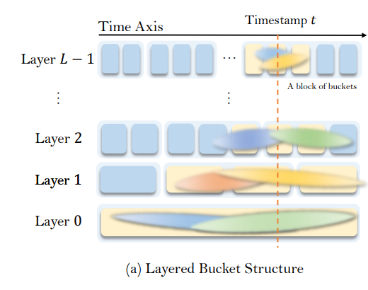
Here, the Layer captures the Gaussian’s duration \(\tau\), while the Bucket captures \(\mu_t\), which indicates where the Gaussian is located along the temporal axis.

Once this is understood, the idea can be summarized as follows:

1. In the original TGH method, if a Gaussian’s time span awkwardly crosses a segment boundary at a given layer level, the Gaussian is moved down to a lower-level layer with a larger temporal segment.
2. This does not directly increase the storage required by the Gaussian itself, but placing a Gaussian with a short temporal extent in a lower layer than it naturally belongs to makes the Gaussian characteristics within that layer less homogeneous and can reduce compression efficiency.
3. In addition, placing Gaussians with different temporal characteristics in the same layer broadens the distribution. This becomes particularly problematic when compressing them with a VQ codebook, which will be discussed later.
4. To address this, the authors reorganize TGH’s fixed-segment structure into a bucket-based structure and allow Gaussians to freely cross bucket boundaries.
5. As a result, even if a Gaussian crosses a Bucket Boundary, its layer does not need to change, allowing it to remain at the layer level appropriate for its temporal characteristics.
6. Moreover, because each layer is divided into multiple buckets, rendering a particular time \(t\) requires loading only the Gaussians from the current bucket and its neighboring buckets onto the GPU. Therefore, even for long videos, only the necessary Gaussians are selectively loaded, guaranteeing visibility while minimizing memory usage.

Rather than manually fixing the number of layers as in TGH, the authors dynamically determine the number of layers \(L\) as follows:

\[L = \lceil \log_2 n \rceil + 1\]

where \(n\) is the total number of frames in the video sequence.

Training Framework

Now we can discuss how to train the Layer-Bucket Structure efficiently. The training framework can be divided into two main components: Triple-buffer training + DARLR.

First, let us explain Triple-buffer training.

As explained earlier, rather than keeping all Gaussians on the GPU at all times, only the Gaussians around the buckets required for timestamp t are used. This means that the timestamp also changes at every training iteration.

In other words, the required set of Gaussians changes whenever a training image is sampled. If the CPU repeatedly copies the required Gaussians to the GPU while the GPU copies unnecessary Gaussians back to the CPU at every iteration, memory transfer between the CPU and GPU becomes a bottleneck. In TGH in particular, this CPU-to-GPU transfer cost is a major bottleneck.

Therefore, the authors use a Triple-buffer. It is a triple-buffer strategy consisting of a GPU double buffer and a CPU bucket buffer.

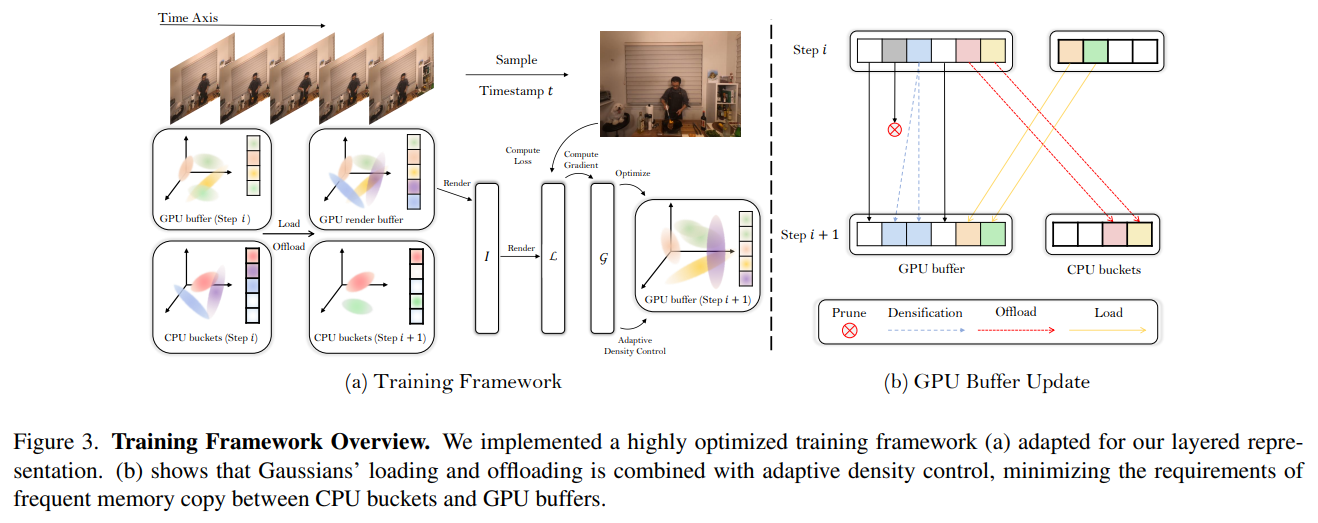
The CPU Bucket Buffer stores all Gaussians in the scene on the CPU according to the bucket structure (Bucket 1, Bucket 2, …). Since Gaussians that are not required at the current timestamp do not need to remain on the GPU, the CPU serves as long-term storage.

The GPU Buffer is the space that keeps Gaussians used in the current or recent iterations on the GPU. As shown in Figure 3(b), the GPU buffer from Step i is not completely cleared; instead, its contents are updated according to the requirements of the next step.

The GPU Render Buffer separately constructs the set of Gaussians actually required to render the current timestamp t.

Now, let us examine how a single training iteration proceeds:

1. Sample one training image at timestamp t
   • From the entire multi-view dynamic video(\(I_0, I_1, I_2, ... , I_t , ... , I_n\)), sample one \(I_t\).
   • This determines the timestamp t to be trained in the current iteration.
2. Update the GPU buffer and construct the GPU render buffer
   • Identify the buckets and Gaussians required at timestamp t.
   • Among the required Gaussians, reuse those already present in the GPU buffer, and load only the Gaussians missing from the GPU from the CPU buckets to construct the GPU render buffer for the current t.
   • At the same time, perform adaptive density control such as pruning and densification.
   • Gaussians that remain on the GPU but have not been used for several steps are offloaded to the CPU buckets.
   • Thus, instead of transferring the entire set of Gaussians back and forth between the CPU and GPU at every iteration, the GPU buffer is continuously maintained while only the necessary Gaussians are loaded and offloaded.
3. Standard 3DGS optimization
   • Once the Gaussians required at the current t are prepared in the GPU render buffer, perform \(Gaussian \rightarrow Render \rightarrow \hat{I}_t\).
   • Compute the Loss by comparing the rendered result \(\hat{I}_t\) with the GT image \(I_t\).
   • Then update the Gaussian parameters through \(Loss \rightarrow Gradient \rightarrow Optimizer\).
   • Among the trained Gaussians, those that should remain on the GPU are carried over to GPU buffer i+1 for the next iteration, while only those that have not been used for a long time are offloaded to the CPU.

Next, let us explain the Dynamic-Aware Rotor Learning Rate (DARLR).

Using a 4D rotor is somewhat different from using Vanilla 3DGS. In Vanilla 3DGS, rotation is purely spatial, so a single rotation learning rate is sufficient. In a 4D rotor, however, temporal components must also be learned. In other words, a 4D rotor contains temporal/spatio-temporal rotor components together with spatial rotation.

If a large learning rate is assigned to the temporal rotor of such a Gaussian, even a small change in temporal orientation during optimization can cause large spatial position drift at times far from the Gaussian’s mean time.

This problem becomes more severe for longer videos because $\lvert t-\mu_t\rvert$ can become much larger.

Therefore, the authors set a smaller temporal-rotor Learning Rate for Gaussians with larger \(\tau\). A large \(\tau\) indicates a Gaussian that persists for a long time and is therefore likely to be static or slowly varying, so reducing the temporal-rotor learning rate suppresses drift over time.

Conversely, short-\(\tau\) Gaussians represent more dynamic regions and can therefore allow relatively larger updates to the temporal rotor.

Factorized Covariance Quantization

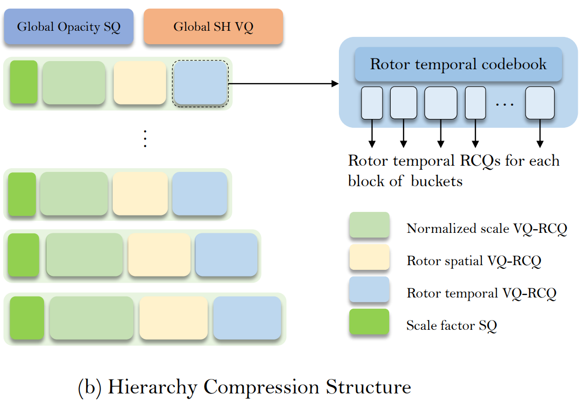
Before discussing the proposed method, let us first review SQ and VQ. Expand the sections below for a brief explanation.

Scalar Quantization

A method that quantizes each scalar value individually

Let us look at an example.

Suppose the value range is \([0,1]\) and 2-bit quantization is used.

Only \(2^2=4\) values can be represented. For example,

\[\{0, 0.33,0.67,1.0\}\]

if only these values are allowed,

\[0.1 \rightarrow 0 \\ 0.4 \rightarrow 0.33 \\ 0.71 \rightarrow 0.67\]

the values are changed as shown above. Naturally, this introduces a small difference from the original value, which is called the quantization error:

\[\text{error} = |x-Q(x)|\]

If every parameter of each Gaussian were originally stored as float32, each value would require 32 bits. Using 8-bit SQ reduces this from 32 bits to 8 bits, thereby lowering storage requirements.

Therefore, SQ is well suited for compressing values such as opacity, scale factors, and other scalar parameters.

In this paper, the scale factor is compressed using SQ, and opacity is also quantized using SQ.

Vector Quantization

This time, instead of quantizing a single number,

\[x = [x_1, x_2, ... , x_D]\]

the goal is to compress an entire D-dimensional vector.

For example, suppose the normalized scale of a Gaussian is

\[s = [0.72, 0.41, 0.19, 0.11]\]

Rather than quantizing each component separately, the entire vector is treated as a single unit.

Suppose the codebook contains the following four vectors.

\[C = \begin{cases} c_1 = [1.0, 0.5, 0.2, 0.1] \\ c_2 = [0.7, 0.4, 0.2, 0.1] \\ c_3 = [0.2, 0.8, 0.6, 0.3] \\ c_4 = [0.1, 0.2, 0.9, 0.7] \end{cases}\]

Comparing the vector with each codebook vector, \(c_1\) would be the most similar. The original vector is therefore not stored; instead, only

\[\text{index} = 1\]

is stored. Later, during rendering, it can be reconstructed using $$c_1$.

Therefore, instead of storing the full float vector for every Gaussian, only a codebook index is stored.

Now that we understand SQ and VQ, let us examine how a 4D Gaussian can be quantized.

The key idea is

Directly applying VQ to the entire covariance of a 4D Gaussian results in a value range that is too large for effective compression. Therefore, the scale and rotor that constitute the covariance are factorized according to their characteristics and quantized separately using suitable methods.

This is the central idea.

We previously examined the following equation:

\[\Sigma_{4D} = R_{4D}S_{4D}S_{4D}^TR_{4D}^T\in \mathbb{R}^{4 \times 4}\]

where

\[S_{4D} = diag(s_x, s_y, s_z, s_t)\]

is the 4D scale of the Gaussian, and

\[R_{4D}\]

is the 4D rotation represented by a 4D Rotor. In other words, the covariance is parameterized by the scale and rotor.

In the previous work “C3DGS,” VQ could be applied directly to normalized 3D covariance. If the covariances of multiple Gaussians were similar, they could share a representative covariance stored in the codebook.

However, the authors argue that VQ cannot be directly applied to 4D covariance because the numerical ranges of the spatial and temporal scales differ too greatly. The paper states that the spatial/temporal scales of 4D Gaussians can span approximately \(10^{-3} \sim 10^3\). This already represents a difference of \(10^6\), and as the equation for \(\Sigma_{4D}\) shows, covariance has a quadratic relationship with scale. Since scale is effectively squared, the range expands further to approximately \(10^{-6} \sim 10^{6}\).

When vectors are distributed across such a wide range, a codebook cannot represent the entire range with sufficient precision, resulting in inadequate VQ representation precision. Therefore, the authors abandon direct VQ of the full 4D covariance and instead introduce Factorized Covariance Quantization. More specifically, the Scale and Rotor are compressed separately.

For Scale, the method first performs Scale Decomposition. The original 4D scale is

\[S_{4D} = (s_x, s_y, s_z, s_t)\]

which contains four values, and it is decomposed into a scale factor and a normalized scale.

Conceptually,

\[s = a\hat{s}\]

where \(a\) acts as the scale factor and \(\hat{s}\) as the normalized scale. These can be understood as representing the overall size of the Gaussian and the relative proportions among its axes, respectively.

The scale factor and normalized scale must then be quantized. Based on the SQ and VQ concepts introduced earlier, the appropriate choice is fairly intuitive: apply SQ to the scale factor and VQ to the normalized scale. The scale factor is a single scalar, so SQ is appropriate, whereas the normalized scale is a vector, which motivates the use of VQ.

Next, let us decompose the Rotor and quantize it.

We previously represented the 4D Rotor \(R_{4D}\) using eight coefficients:

\[(s, b_{01}, b_{02}, b_{12}, b_{03}, b_{13}, b_{23}, p)\]

We interpreted the first four coefficients as the spatial component and the last four as the temporal/spatio-temporal component.

The authors make an intuitive observation here. For a static Gaussian such as one representing a wall, the spatial rotor should behave similarly to an ordinary quaternion, while the temporal rotor component is expected to remain close to zero. This provides a natural way to separate static and dynamic behavior: static Gaussians still require spatial orientation, but they require little space-time rotation, so their temporal components are likely to be small.

If VQ is applied to the entire 8D rotor at once, the value ranges (distributions) of the first four and last four coefficients differ substantially, forcing a single codebook to represent two types of statistics simultaneously and making quantization more difficult.

\[Rotor \rightarrow Rotor_{spatial}+Rotor_{temporal}\]

After this decomposition, separate VQ codebooks are assigned to the spatial rotor and temporal rotor. As a result, only

\[i_{spatial}, i_{temporal}\]

two indices need to be stored.

During decoding, these indices are used to retrieve the spatial and temporal rotor components from their respective codebooks. The two components are then merged and normalized to recover the full rotor.

In addition, following C3DGS, the authors use Gaussian importance weights. They render all training images over time, measure how much each Gaussian contributes to pixels using backpropagation gradients, and use this value as the quantization weight.

Layered Compression

We have now decomposed the covariance into the scale factor, normalized scale, rotor spatial component, and rotor temporal component, and the goal is to compress these components using codebooks.

The key idea is not to compress these components for all Gaussians using a single codebook, but instead to compress them separately for each temporal layer. In other words,

Since Gaussian parameter distributions differ across layers, use a separate codebook for each layer

In the Layer-Bucket structure described earlier, Gaussians are assigned to different layers according to their temporal extent \(\tau\). Therefore, the distributions of these components can differ across Gaussians with different temporal extents, that is, across different layers.

If all layers are compressed using a single VQ codebook, the codebook must simultaneously cover very different distributions. This either requires many representative vectors, increasing the codebook size, or, if the codebook is kept small, increases the quantization error. In other words,

Using a shared codebook increases codebook size and quantization error because of the wide distributional variance.

Therefore, the authors perform layer-wise compression.

Each layer is assigned its own codebook: codebook 0 for layer 0, codebook 1 for layer 1, and so on. Each codebook therefore needs to represent only the narrower distribution of its own layer.

However, parameters such as Gaussian SH coefficients and Opacity use Global VQ and Global SQ, respectively.

Opacity is naturally bounded after the sigmoid, with \(\alpha \in [0,1]\), while the distribution of SH coefficients remains relatively consistent across layers. Therefore, a single global codebook is sufficient to represent SH coefficients across all layers, reducing storage requirements.

Thus, because separate codebooks are used for Normalized scale, rotor spatial, and rotor temporal in each layer, these account for \(3L\) codebooks, and the global SH codebook adds one more, giving \(3L+1\) codebooks in total. The remaining components use SQ and therefore do not require codebooks. If the number of quantization units is counted including SQ, the total becomes \(4L+2\). In addition, the paper also merges some of the layers themselves.

Not all layers contain many Gaussians, so the later layers with relatively few Gaussians are merged together. This reduces the overhead associated with maintaining separate codebooks.

Residual Codebook Quantization (RCQ)

The authors construct a separate VQ codebook for each layer. However, for extremely long videos, the parameter distributions of Gaussians can differ even within the same layer when they are far apart in time. In this case, a single codebook per layer may have insufficient capacity to represent the entire layer. The paper refers to this as a limited capacity problem.

Therefore, the Gaussians in the buckets of each layer are further divided into multiple bucket blocks. If a layer contains Blocks A, B, and C, then separate codebooks A, B, and C are constructed for those blocks, yielding more localized distributions.

However, storing a full codebook for every block would increase storage again.

Therefore, instead of storing each entire codebook, the method stores only the difference.

Let the existing codebook for the entire layer be \(C_{global}\), and let the codebook optimized for a specific block be \(C_{block}\).

\[C_{block} \approx C_{global} + \Delta C\]

Here, \(\Delta C\) is referred to as the residual.

Instead of storing the entire block-specific codebook, the authors quantize the difference between that codebook and the layer-global codebook again using a residual codebook. In this sense, the Gaussians undergo two stages of compression: the layer-global codebook provides the coarse representation, while the residual codebook quantizes the distribution of differences between the layer-global and block-specific codebooks.

The order can be confusing, so the process can be summarized more clearly as follows:

Perform a separate VQ for the Gaussians in each Block to construct a block-specific codebook \(C_{block}\). Then compare it with the existing layer-global codebook \(C_{global}\) to obtain the residuals. Finally, quantize these residuals again using a small residual codebook.

This makes it possible to discard the block-specific codebook and reconstruct it again during decoding as

\[\hat{C}_{block} = C_{global} + C_{residual}\]

which reconstructs the block-specific codebook.

Thus, Gaussians in a particular block can be decoded using the stored global codeword index and Residual codeword index.

This also shows that an index table is required. In practice, rather than storing a separate residual codebook for every block, the method uses a lightweight residual representation together with an index table to reduce overhead, because otherwise the storage requirements could increase substantially.

RCQ is also not applied to Layer 0. The authors report that Layer 0 generally exhibits less temporal variation and therefore benefits less from additional local residual compression.

Experiments

Implementation Details

The authors use a single NVIDIA RTX 3090. Training takes approximately 30 minutes while using only 2 GB of GPU memory, and compression takes about 4 minutes. During inference, rendering is sustained at 660 FPS.

Datasets

The authors evaluate on the N3DV and SelfCap datasets. N3DV contains six dynamic scenes, each captured for 10 seconds using 19~21 cameras at a resolution of 1352 \(\times\) 1014. SelfCap contains six scenes featuring large motions, and its sequences are characterized by long durations of 1~10 minutes.

Evaluation on N3DV Dataset

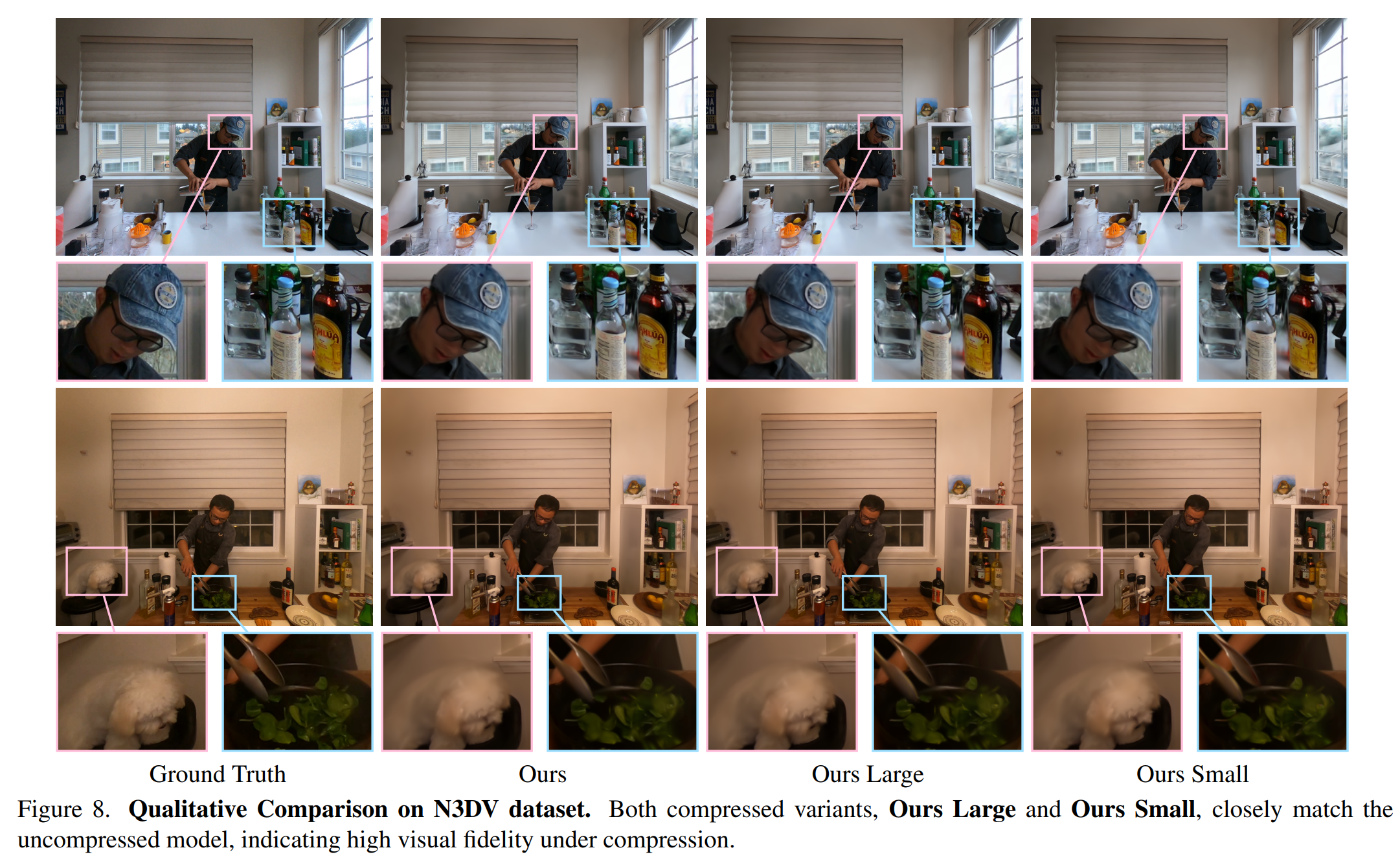
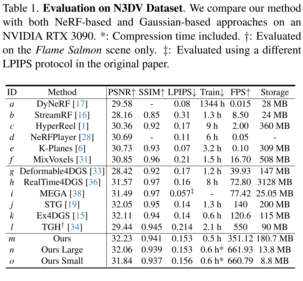
Table 1 compares the method with existing NeRF-based and Gaussian-based approaches. The Ours model is the uncompressed version, which provides high visual quality but requires relatively large storage. Ours Large reduces storage by 13.1× after a 4-minute compression stage and achieves approximately 90% faster rendering while introducing only a minor performance drop. Ours Small further increases the compression ratio to 20.5×, reducing the bitrate to below 1 MB/s while still maintaining visual quality comparable to existing baselines.

Evaluation on SelfCap Dataset

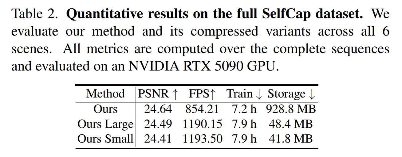
Most Dynamic NVS baselines can process only short clips of around 10 seconds. To evaluate effectiveness on long video sequences, the authors evaluate all six SelfCap scenes.

As shown in Table 2, compression preserves visual quality while reducing storage requirements and substantially improving rendering efficiency, resulting in an approximately 40% increase in FPS. Ours Large provides high-fidelity reconstruction, while Ours Small increases the compression ratio to 19.1× while maintaining competitive visual quality.

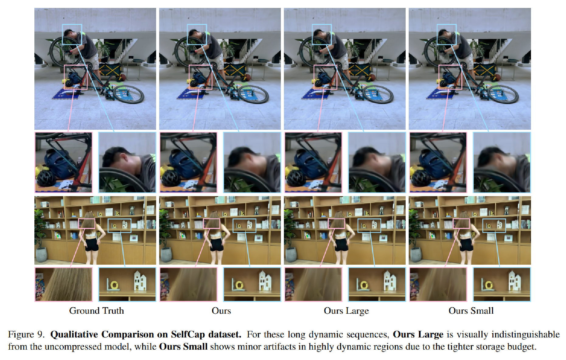
As shown in Figure 9, the method preserves high-frequency details and high fidelity even in regions containing highly dynamic and rapid interactions between people and objects. The compressed results also remain very similar to those produced by the original uncompressed model.

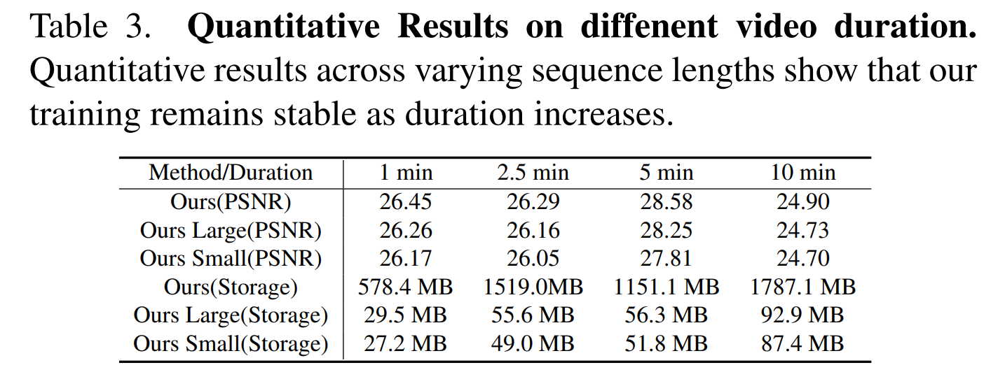
Furthermore, the authors use the SelfCap Bike scene to evaluate reconstruction performance on even longer sequences. As shown in Table 3, the method maintains consistently stable performance as the video duration increases.

Ablation Studies

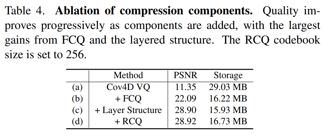
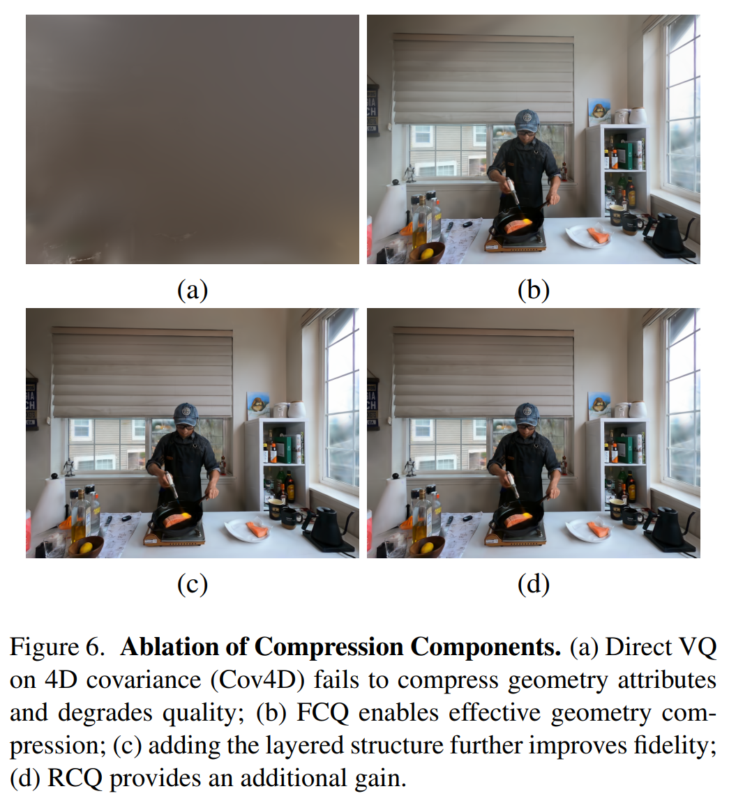
On the N3DV Flame Salmon scene, the authors progressively remove the key design components of the Compression pipeline and measure the resulting changes in quality and performance. As indicated by the PSNR results in Table 4 and Figure 6, directly quantizing the 4D covariance causes a severe drop in reconstruction fidelity. Applying FCQ both reduces storage and improves PSNR. Adding Layered Compression further improves PSNR. Finally, adding RCQ provides additional quality recovery by refining the quantized representation, at the cost of only a small increase in storage.

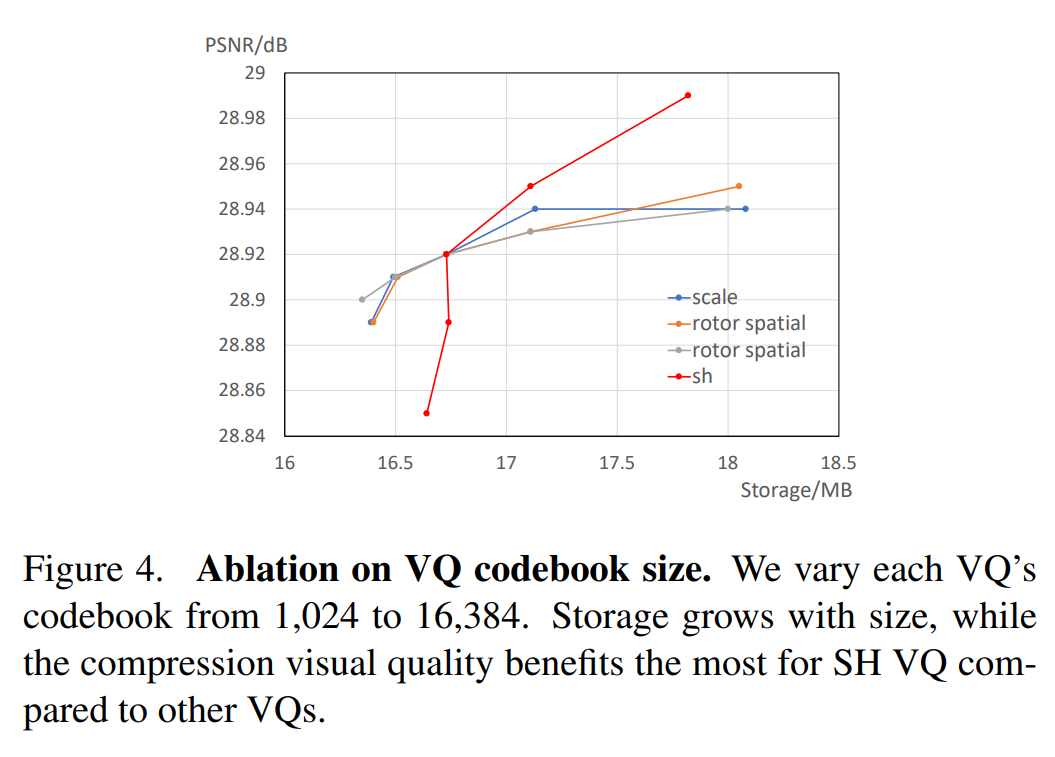
The authors also analyze the effects of the main hyperparameters of the compression algorithm on the N3DV Flame Salmon scene. As shown in Figure 4, progressively increasing the VQ codebook size from 1024 to 16384 reduces Compression error and consistently improves PSNR, but also increases storage requirements. In particular, increasing the SH codebook size yields the strongest quality improvement per unit of storage (PSNR per MB).

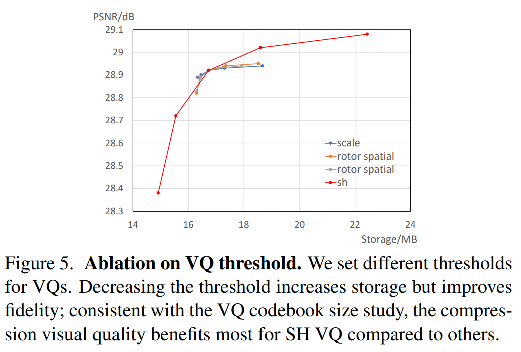
Figure 5 shows the trade-off between storage efficiency and visual quality when the VQ threshold for SH features is lowered to quantize them more precisely.

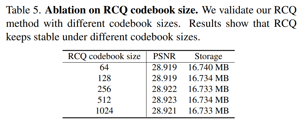
Table 5 shows that varying the RCQ codebook size across multiple settings causes only minor changes in the final storage size and visual quality, demonstrating the model’s robustness to this parameter.

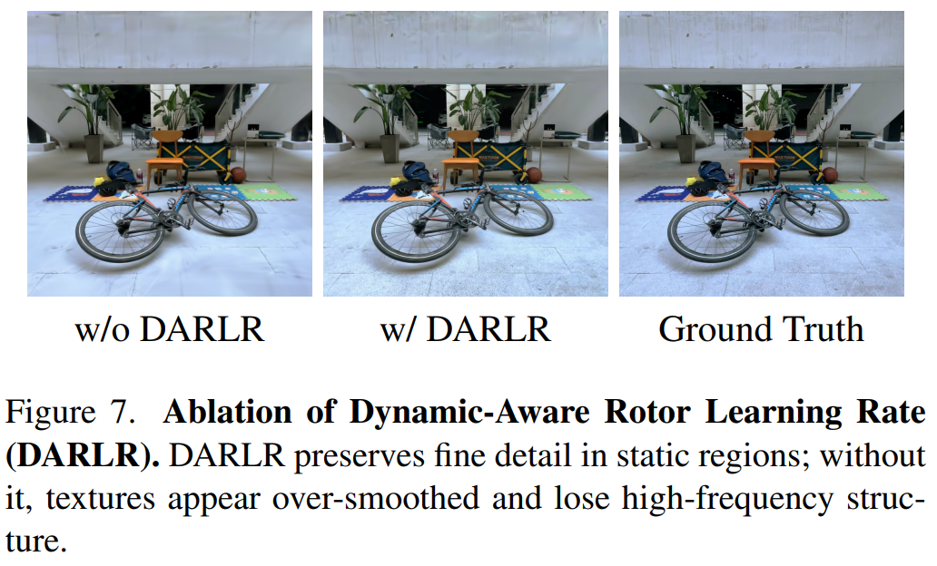
The authors apply the DARLR strategy during training, and the results show that it preserves fine textures and structures in static background regions sharply without blurring.

Limitations & Future work

1. Although the proposed pipeline achieves very low VRAM usage, the process of compressing the trained Gaussians itself requires a considerable amount of time.
2. The method does not support online training that can incorporate incoming video sources in real time.

Therefore, future work should investigate faster compression methods and frameworks that support real-time online training and progressive compression.