[Paper Review, EN] Lyra: Generative 3D Scene Reconstruction via Video Diffusion Model Self-distillation

Paper Information
Title: Lyra: Generative 3D Scene Reconstruction via Video Diffusion Model Self-distillation
Authors: Sherwin Bahmani, Tianchang Shen, Jiawei Ren, Jiahui Huang, Yifeng Jiang, Haithem Turki, Andrea Tagliasacchi, David B. Lindell, Zan Gojcic, Sanja Fidler, Huan Ling, Jun Gao, Xuanchi Ren
Venue: ICLR 2026
Link: [Paper], [Project], [Github]

Teaser Image

Introduction

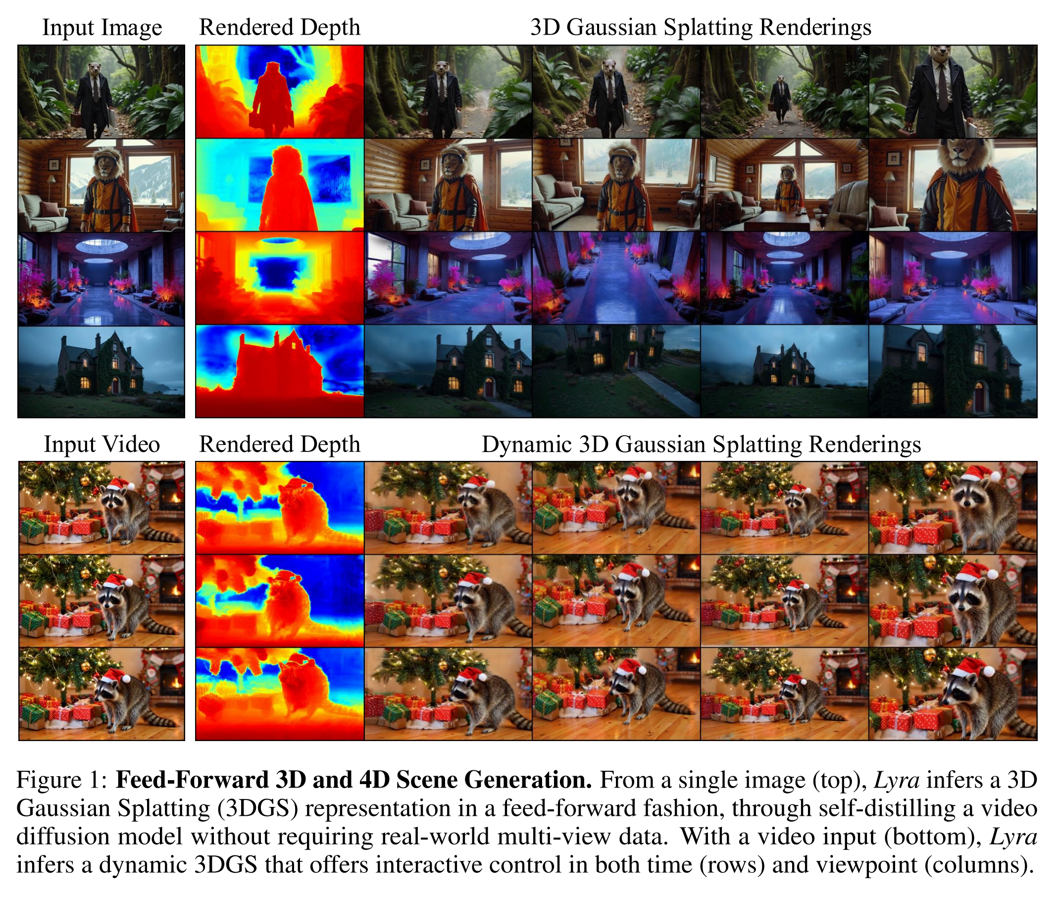
3D scene reconstruction has achieved high quality through advances in NeRF and 3D Gaussian Splatting (3DGS), but it still relies heavily on accurate camera poses and multi-view images. Dynamic scenes require synchronized multi-camera capture as well, which further increases the burden of data collection. Meanwhile, 3D generation has advanced through optimization-based approaches that leverage CLIP and diffusion priors, but these methods require repeated optimization for each scene.

Subsequently, methods emerged that generate novel views with multi-view diffusion and then reconstruct them with NeRF or 3DGS, as well as feed-forward reconstruction methods that directly predict a 3D representation from an image or text. However, the former still requires per-scene optimization, while the latter relies on limited multi-view datasets such as RealEstate10K or DL3DV, which restricts generalization.

Recently, as large-scale video diffusion models have learned diverse scenes and camera motions, camera-conditioned video generation and multi-view consistency have advanced rapidly. As a result, connecting the implicit 3D/4D knowledge of video diffusion models to explicit 3D representations has become an important research direction.

Method & Technical Details

I will start with the core idea.

The goal is to distill the implicit 3D knowledge embedded in a video diffusion model into an explicit 3DGS decoder.

The two most important components in distillation, the teacher and the student, are respectively the video diffusion model and a 3DGS decoder that operates in latent space. The framework is also built upon GEN3C, a recently developed camera-conditioned video diffusion model.

Background: Camera-controlled and 3D-Consistent Video Diffusion

Since this work is built upon GEN3C, I think it is useful to understand, at least to some extent, how the teacher model GEN3C generates camera-controlled videos.

Spatiotemporal 3D Cache

In GEN3C, the input image/video is not simply fed directly into the video diffusion model. Instead, the depth of each frame is first estimated, and the RGB pixels are unprojected into a 3D colored point cloud using the estimated depth.

The paper denotes this as

\[P_{t,v}\]

Here, $t$ denotes the frame index and $v$ denotes the viewpoint. Therefore, $P_{t,v}$ can be understood as the colored 3D point cloud obtained at time $t$ from viewpoint $v$.

Given an RGB image $I_{t,v}$ and its corresponding depth map, each pixel $(u,v)$ can be approximately mapped as

\[x = D(u,v)K^{-1} \begin{bmatrix} u \\ v \\ 1 \end{bmatrix}\]

Using depth, the 3D position can be recovered in this way, and attaching the original RGB color yields a colored point cloud. The collection of these point clouds stored according to time and viewpoint forms the spatiotemporal 3D cache $P_{t,v}$. The paper describes it as an $L \times V$ structure:

\[\begin{array}{c|cccc} & v_1 & v_2 & \cdots & v_V \\ \hline t_1 & P_{1,1} & P_{1,2} & \cdots & P_{1,V} \\ t_2 & P_{2,1} & P_{2,2} & \cdots & P_{2,V} \\ \vdots & & & & \\ t_L & P_{L,1} & P_{L,2} & \cdots & P_{L,V} \end{array}\]

A convenient way to think about this is that, instead of asking the video diffusion model to internally remember the entire scene structure, GEN3C constructs an external scene memory in explicit 3D form.

Rendering and structured guidance

The next key step is to re-render the point cloud along a camera trajectory specified by the user.

\[(I^{t,v}, M^{t,v}) = R(P^{t,v}, C^t)\]

Here, $C^t$ is the target camera pose we want, and $R$ is the point cloud renderer. In other words, this means viewing the 3D point cloud created from the original viewpoint through a new target camera $C^t$.

However, this introduces a problem. A single-view point cloud does not contain the surfaces hidden behind foreground objects. Therefore, when the camera view changes and a previously occluded region becomes visible, that region may be empty. This phenomenon is referred to as disocclusion.

For this reason, the GEN3C renderer outputs not only an RGB rendering but also a disocclusion mask $M^{t,v}$. We therefore have three forms of guidance:

Rendered RGB + Disocclusion mask + Target Camera Trajectory

These are provided to the video diffusion model as structured guidance. The video diffusion model then preserves regions already known from the 3D cache as much as possible, generates content for missing regions indicated by $M$, and produces a temporally continuous video following the camera trajectory.

GEN3C is better suited to maintaining 3D consistency than a conventional camera-conditioned video diffusion model because it does not provide only numerical camera poses; instead, it directly renders the current scene geometry and supplies it as visual guidance.

If we denote the Camera Trajectory as

\[C = (C_1, C_2, ... , C_L)\]

then the above process is performed for each camera pose.

For viewpoint $v$, this produces

\[I^V \in \mathbb{R}^{L \times 3 \times H \times W}\]

an RGB image sequence and

\[M^V \in \mathbb{R}^{L \times 1 \times H \times W}\]

a mask sequence.

This entire sequence becomes camera-aware guidance for the video diffusion model.

Video variational autoencdoer(VAE)

This part is not intended to explain another idea from GEN3C, but rather to clarify the representation that Lyra will use later.

A typical video diffusion model does not perform diffusion directly in the original RGB video space. Instead, it operates in a compressed latent space obtained using a VAE encoder.

If the RGB video is written as

\[I \in \mathbb{R}^{L \times 3 \times H \times W}\]

then the VAE encoder $E$ transforms it as

\[z = E(I)\]

The resulting latent is

\[z \in \mathbb{R}^{L' \times C \times h \times w}\]

In GEN3C/Lyra, $C=16$, and since the spatial compression factor is $\sigma = 8$,

\[h = \frac{H}{8}, w = \frac{W}{8}\]

The temporal dimension is also compressed by $\tau=8$, giving

\[L'=\frac{L-1}{8}+1\]

Finally, once the diffusion model generates the latent $z$, the pretrained RGB decoder

\[\hat{I} = D_{rgb}(z)\]

reconstructs it back into a video. The latent $z$ is particularly important because Lyra does not simply use the RGB video generated by GEN3C; instead, it directly decodes 3DGS from the video latent $z$ before that latent is decoded into RGB.

Self-Distillation

Now I will discuss how the 3DGS decoder is trained using GEN3C. More precisely,

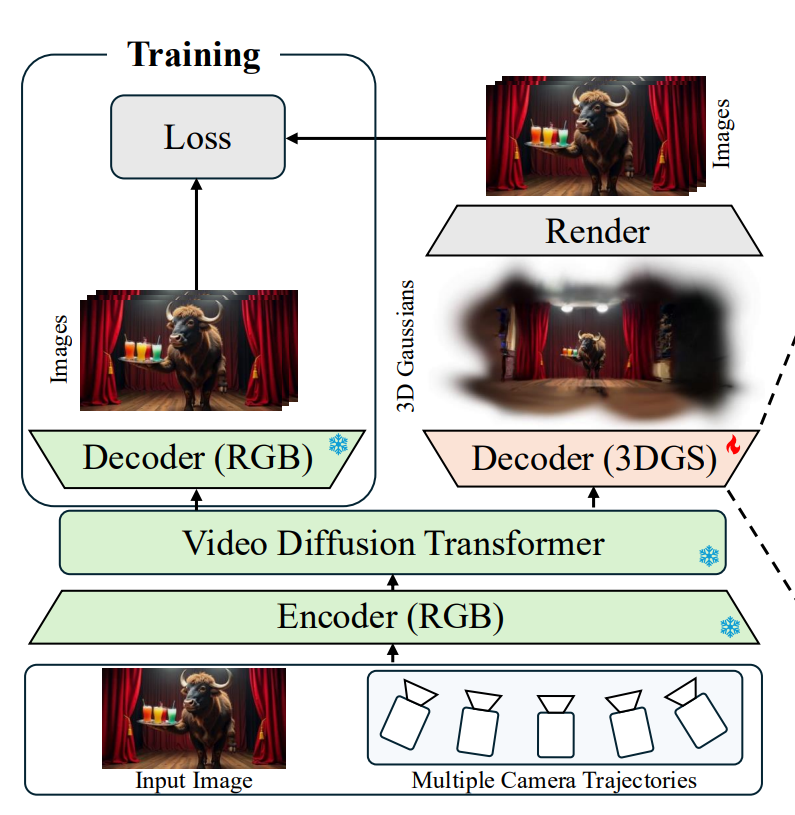
GEN3C generates RGB videos from multiple camera views, and Lyra trains its 3DGS decoder to reproduce those videos through a 3DGS representation.

Before that, we first need to understand why self-distillation is necessary.

Conventional feed-forward 3D reconstruction typically requires data in the form of {multi-view images, camera poses}. The problem is that the diversity of such real multi-view datasets is limited. Lyra therefore takes the approach of not collecting real multi-view data, but instead letting a video diffusion model already trained on extremely diverse video data generate the multi-view training data.

First, Lyra uses an LLM to create diverse text prompts. For example, it generates many prompts such as “a living room with a large window,” and then uses an image diffusion model to generate an image $I$. This single image $I$ is fed into GEN3C, which generates videos along multiple camera trajectories. In other words, GEN3C provides synthetic multi-view supervision.

Let us denote GEN3C as $V$. Then the input image $I$ and camera trajectory ${C_t}_{t=1}^L$ are fed into GEN3C:

\[z = V(I, \{C_t\}_{t=1}^L)\]

This produces the latent $z$, which is decoded along two branches:

1. RGB decoder
2. 3DGS decoder

As the Teacher, the pretrained RGB decoder $D_{rgb}(z)$ originally included in GEN3C

\[I_{D_{rgb}(z)} = D_{rgb}(z)\]

produces an RGB video. This serves as the teacher target.

As the Student, Lyra feeds the same $z$ into the newly added 3DGS decoder $D_s$:

\[G = D_s(z)\]

Here, $G$ denotes the 3D Gaussians. Thus, the video latent $z$ can ultimately be transformed into both an RGB video and 3D Gaussians.

The problem is that an RGB video and a 3DGS representation cannot be compared directly, so the student 3DGS $G$ is rendered:

\[I_{D_s} = Render(G, \{C_t\}_{t=1}^L)\]

This produces 2D images from the same camera poses as the teacher, and

\[I_{D_s} \approx I_{D_{rgb}}\]

$D_s$ is trained so that this relationship holds.

At first glance, this may seem a little strange: “Why is this called self-distillation? Isn’t it just distillation?” Based on the discussion above, we can think of it as follows:

\[\text{Student Render} = \text{Teacher RGB}\]

The key point, however, is that both branches start from the same latent $z$ and share this latent representation. In other words, the information encoded by the video diffusion model is distilled from the implicit 3D knowledge in the video latent $\rightarrow$ explicit 3D Gaussians.

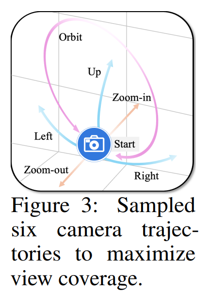
Additionally, Lyra samples six camera trajectories for each input image ($V=6$). Each trajectory contains $L=121$ camera poses. Thus, it can generate frames corresponding to a total of $6 \times 121 = 726$ viewpoints.

Importantly, Lyra does not construct a separate 3DGS for each of the six trajectories. A simple approach could be

\[\begin{aligned} z^1 \rightarrow G^1 \\ z^2 \rightarrow G^2 \end{aligned}\]

where one 3DGS is created for each trajectory, but Lyra instead takes the latents from all six trajectories

\[Z = \{z^1, ... , z^6\}\]

and jointly produces a single coherent 3DGS $G$. In other words,

\[\{z^1, ... , z^6\} \rightarrow D_s \rightarrow G\]

This is what the paper refers to as multi-view fusion. Once the Gaussian Scene $G$ has been constructed, it can be rendered from every camera in all six trajectories. These renderings are then compared with the corresponding RGB frames generated by the GEN3C teacher.

\[I^{t,v}_{D_s} \approx I^{t,v}_{D_{rgb}}\]

As a result, the single 3D scene produced by the student must simultaneously match the teacher videos across multiple camera trajectories.

It is also important to consider which components are updated during training. According to the architecture figure, the pretrained video diffusion model and the RGB VAE encoder/decoder are frozen, and only the 3DGS Decoder $D_s$ is trained. At inference time, GEN3C is still needed to produce the latent $z$; only its RGB decoder becomes unnecessary.

3DGS Decoder

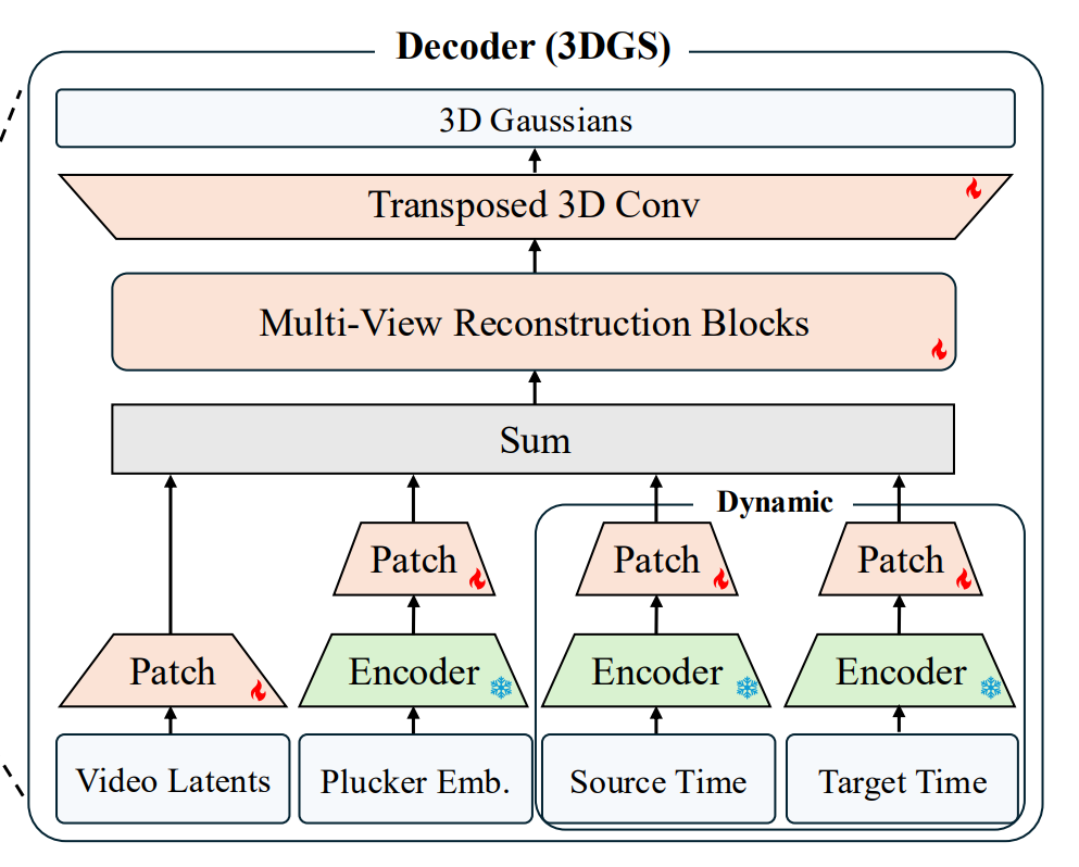
Now we can look at the Architecture of the 3DGS Decoder, which can be considered one of Lyra’s core contributions.

First, consider the input to the 3DGS decoder. As calculated earlier, there are 726 views in RGB space, and each frame has a resolution of $704 \times 1280$. Existing feed-forward reconstruction models generally cannot process this many images at once. The main problem is that converting every image pixel into a visual token and applying attention makes the number of tokens, memory usage, and computation prohibitively large.

Therefore, instead of feeding 726 RGB images into the decoder, Lyra directly uses the latent representation already compressed by the video diffusion model. The video latent for a single trajectory is approximately

\[z^v \in \mathbb{R}^{L' \times C \times h \times w}\]

Collecting all six trajectories gives

\[Z \in \mathbb{R}^{V \times L' \times C \times h \times w}\]

In Lyra, $V=6, L=121$, and the VAE compression factor is 8 in both the temporal and spatial dimensions, so

\[L' = \frac{121-1}{8}+1= 16, h= \frac{704}{8} = 88, w= \frac{1280}{8} = 160\]

Therefore, although the original representation would require handling $6 \times 121 \times 704 \times 1280$ dense image elements, the video latent actually processed by the decoder is approximately

\[Z \in \mathbb{R}^{6 \times 16 \times 16 \times 88 \times 160}\]

In other words, Lyra’s Latent-Based 3D Reconstruction performs reconstruction only after heavily compressing both the temporal and spatial dimensions with the VAE.

This gives us one of the inputs used by the 3DGS Decoder. The other input is camera information. Here, Lyra uses a technique called Plücker embedding, which has also appeared frequently in my previous review posts.

More precisely, it represents information about the camera ray from which a feature was observed. Lyra therefore uses the Plücker embedding $E$ as the second input.

\[G = D_s(Z,E)\]

which defines the static decoder.

Briefly, the raw Plücker embedding is computed from the camera pose and intrinsics as

\[E_{raw} \in \mathbb{R}^{V \times L \times 6 \times H \times W}\]

Thus, there is one camera-ray descriptor for every trajectory, every frame, and every pixel. Conceptually, the reconstruction network receives, for each pixel, the visual feature + information about the ray from which that feature was observed.

However, the Plücker embedding is at full resolution, while $Z$ is at latent resolution.

\[Z \in \mathbb{R}^{V \times L' \times C \times h \times w} \\ E_{raw} \in \mathbb{R}^{V \times L \times 6 \times H \times W}\]

Their sizes are therefore completely different. Lyra addresses this by reusing the RGB encoder of the pretrained video VAE for the Plücker embedding as well. The Plücker representation has 6 channels, whereas the RGB encoder normally expects a 3-channel input. The 6-dimensional Plücker representation is therefore split into two 3-dimensional components:

• 3D ray direction
• the 3D component corresponding to the cross-product of the ray direction and ray origin

Each component is passed through the VAE encoder separately and then concatenated, yielding

\[E_{enc} \in \mathbb{R}^{V \times L' \times 2C \times h \times w}\]

The Plücker latent therefore has $2C$ channels, whereas the video latent $Z$ has $C$ channels, so a lightweight MLP reduces it to $C$ channels.

As a result,

\[E \in \mathbb{R}^{V \times L' \times C \times h \times w}\]

Now $Z$ and $E$ have the same shape. Adding them as $X=Z+E$ can be interpreted as injecting geometry information into each video latent feature, indicating which camera ray that feature corresponds to.

At this point, $Z,E$ are ready. However, they are not fed directly into the Transformer; an additional Patchification step is applied. A $2 \times 2$ patchification layer is applied separately to $Z$ and $E$, converting the video latents into flattened tokens that can be processed by the reconstruction network.

This reduces the number of tokens while simultaneously projecting each patch into a feature vector that matches the hidden dimension of the reconstruction network. The resulting features are then summed and passed into the reconstruction block.

Thus, Patch(Z) + Patch(E) becomes the input to the reconstruction blocks. The next task is to mix information from all six trajectories. In other words, the goal is to construct one coherent 3D scene from $z^1, z^2, … , z^6$. This role is handled by the Multi-view reconstruction blocks inside the 3DGS decoder architecture.

Following Long-LRM, Lyra constructs each block from one Transformer and seven Mamba-2 layers. This block is repeated twice, resulting in 16 layers with a hidden dimension of 512.

Why, then, are Transformer and Mamba-2 combined?

Transformer self-attention becomes extremely expensive in both computation and memory for long sequences. In contrast, Mamba-2 can process long sequences much more efficiently.

The Appendix experiments also show that, under the same setting, the joint Transformer-Mamba architecture is substantially faster than Transformer-only. The paper explicitly states that this design is adopted from Long-LRM.

After passing through the Multi-view reconstruction blocks, the hidden features are complete. Finally, Transposed 3D Convolution expands them back toward the spatial/temporal resolution and decodes them into Gaussian parameters.

The final output is therefore

\[G \in \mathbb{R}^{V \times L \times H \times W \times 14}\]

which the paper describes as per-pixel 3D Gaussian features. To see why there are 14 channels,

• 3D position: \((x, y, z)\)

• Scale: \((s_x, s_y, s_z)\)

• Rotation quaternion: \((q_w, q_x, q_y, q_z)\)

• Opacity: \(\alpha\)

• RGB color: \((r, g, b)\)

Thus, the total number of parameters is

\[3 + 3 + 4 + 1 + 3 = 14\]

The phrase per-pixel 3D Gaussian features may make it sound as though one Gaussian is generated for every pixel, but the Appendix states that the implementation actually generates only one Gaussian for each spatial $8 \times 8$ pixel neighborhood. With only a few viewpoints this could leave too few Gaussians and make the scene look sparse, but Lyra uses a very large number of viewpoints, so this is not a major issue. The number is further reduced through opacity pruning. In other words, the actual implementation performs spatial subsampling.

Loss Function

This section explains how the Gaussians predicted by the 3DGS decoder are matched to the outputs of the GEN3C teacher.

\[L = \lambda_{mse}L_{mse} + \lambda_{lpips}L_{lpips} + \lambda_{depth}L_{depth} + \lambda_{opacity}L_{opacity}\]

As mentioned earlier, the loss is not applied directly to the parameters of $G$. Instead, it is computed from images obtained by rendering $G$ from camera $C$. The MSE loss matches RGB values at the pixel level. However, although MSE is effective at directly matching pixel values, it does not sufficiently capture human-perceived texture or perceptual similarity, so Lyra also uses an LPIPS loss.

LPIPS uses VGG as its feature extractor. Thus, while MSE compares pixels against pixels, LPIPS can be thought of as comparing visual features against visual features.

However, using only these two losses leads to another problem.

Training the 3DGS decoder using only RGB losses produces flattened geometry.

To address this, the authors add another loss term. Lyra uses an off-the-shelf system called ViPE to estimate consistent video depth for the teacher video.

\[D_{teacher} = ViPE(I_{teacher})\]

This provides depth supervision, which is compared with $D_{student}$. Rather than using a simple depth MSE, Lyra adopts the Scale-Invariant depth loss from Long-LRM. This encourages the relative depth structure to match rather than enforcing the absolute depth scale itself. In other words, it helps the model match the structure of the depth map rather than exact depth values.

Lyra also uses an Opacity loss to reduce unnecessary Gaussians. Specifically, it applies L1 regularization to Gaussian opacity, encouraging many Gaussian opacities to approach zero so that unimportant Gaussians satisfy $\alpha_i \rightarrow 0$.

This makes opacity sparse during training, after which the 80% of Gaussians with the lowest opacity are removed. Thus, $L_{opacity}$ is directly connected to pruning.

As the ablation results also show, this reduces rendering time.

The $\lambda$ values for the individual loss terms are

\[\lambda_{mse} = 1.0, \; \lambda_{lpips} = 0.5, \; \lambda_{depth} = 0.05, \; \lambda_{opacity} = 0.1\]

respectively.

Extension to Dynamic 3D Scenes

We have so far constructed the static Lyra Architecture, which can effectively generate Scenes for static environments. The next step is to extend this Architecture to Dynamic Scenes.

In Static Lyra, the input was a single image $I$. Now, however, the input is

\[I_1, I_2, ... , I_L\]

a monocular video. What we want now is not a single $G$, but a time-varying 3D scene

\[G_t\]

The basic self-distillation structure remains almost identical to the static case.

First, given an input video, GEN3C generates videos from different camera viewpoints while preserving the same underlying motion. In other words, it creates synthetic multi-view videos that observe the same motion from multiple viewpoints.

The training videos are also obtained without collecting real synchronized multi-camera data. Instead, prompts are generated with an LLM, videos are synthesized using video diffusion models such as Cosmos or Wan, and camera poses and depth are annotated with ViPE.

In static Lyra,

\[G = D_s(Z,E)\]

whereas in the Dynamic setting,

\[G = D_d(Z,E,T_{src}, T_{tgt})\]

two time conditions are added. They indicate, respectively, the motion state corresponding to each input video frame and the time at which the 3DGS scene to be generated should exist.

In other words, $T_{src}$ tells the Dynamic decoder which time each frame corresponds to, while $T_{tgt}$ specifies the timestep of the 3D scene that should be generated.

The decoder then generates a 3DGS $G_{T_{tgt}}$. Importantly, Time is not passed simply as a scalar value; it is encoded into the same shape as the video latent before being provided to the decoder.

The raw source time is

\[T_{src, raw} \in \mathbb{R}^{V \times L \times 1 \times H \times W}\]

The target time corresponds to a single target timestep, so

\[T_{tgt, raw} \in \mathbb{R}^{V \times 1 \times 1 \times H \times W}\]

However, the RGB VAE encoder expects a 3-channel input. Therefore, the scalar time value is augmented with a 2-dimensional sinusoidal embedding to produce 3 channels.

Conceptually, this is approximately

\[t \rightarrow [t, sin(\cdot), cos(\cdot)]\]

This can be understood as a 3-channel representation of time. Passing it through the pretrained RGB encoder gives

\[T_{src}, T_{tgt} \in \mathbb{R}^{V \times L' \times C \times h \times w}\]

which has the same shape as the video latent. The Target time is repeated across the entire latent temporal dimension $L’$. This is easy to see in the 3DGS decoder architecture figure.

The dynamic decoder is not trained from scratch. Instead, the static decoder $D_s$ is used to initialize $D_d$, which is then fine-tuned. The patchification layers for $T_{src}, T_{tgt}$ are zero-initialized so that the behavior of the static network is not disrupted and the model initially relies primarily on $Z+E$. During training, it gradually learns to use the time conditioning.

When training the Dynamic decoder, the model does not supervise 3DGS representations for all $L$ timesteps at once. Instead, one target timestep is randomly sampled. The Gaussian Scene for that timestep is rendered from multiple cameras, and those renderings are compared against the corresponding teacher frames at the same time.

This can lead to imbalanced viewpoint coverage. In the static pipeline, a single $G$ can use frames from all timestamps, so both near and far views can contribute to supervision. In the dynamic case, however, supervision is restricted to frames corresponding to the randomly sampled timestep, which may expose the model mostly to near views or mostly to far views. The w/o data augmentation example in the figure below illustrates this issue.

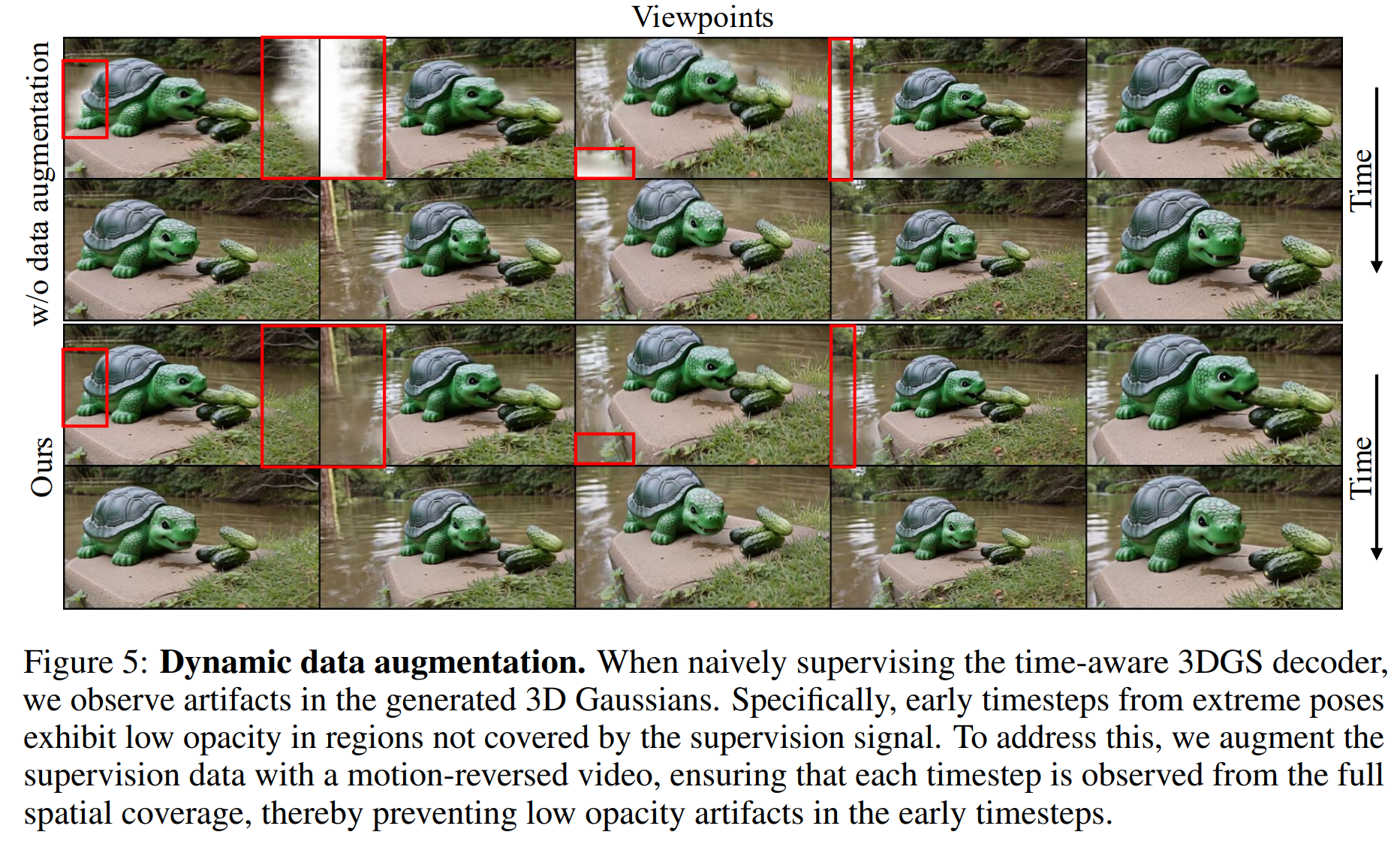
This issue is also related to Lyra’s opacity regularization, which can prune Gaussians that contribute very little from the supervised view.

To address this, Lyra uses a special augmentation strategy. If the input video is $I_1, … , I_L$, the frame order is reversed to obtain $I_{L}, … , I_1$, and this reversed video is fed into GEN3C again. As a result, even for a particular timestep, supervision is available from viewpoints corresponding to both the original temporal direction and the reversed temporal direction. GEN3C generates six additional trajectories for the reversed sequence. After the generated sequences are reversed back to the original motion order, these trajectories effectively provide far-to-near views, complementing the six original near-to-far trajectories. Thus, for any given $G$ at a particular timestep, 6 near views and 6 far views can be used together.

This ultimately provides 12 supervision views per timestep. The effect can be seen in Ours in Figure 5 above. Importantly, this augmentation is used only during training.

Experiments

Setup

No existing multi-view dataset is used to train the model. Instead, Lyra constructs its own Lyra dataset and trains the 3DGS decoder on it. The data are generated from diverse text prompts and span indoor and outdoor environments, humans, animals, and both realistic and imaginative content.

For evaluation, benchmarks such as RealEstate10K, DL3DV, and Tanks and Temples are used, following the same evaluation protocol as Wonderland.

Main Results

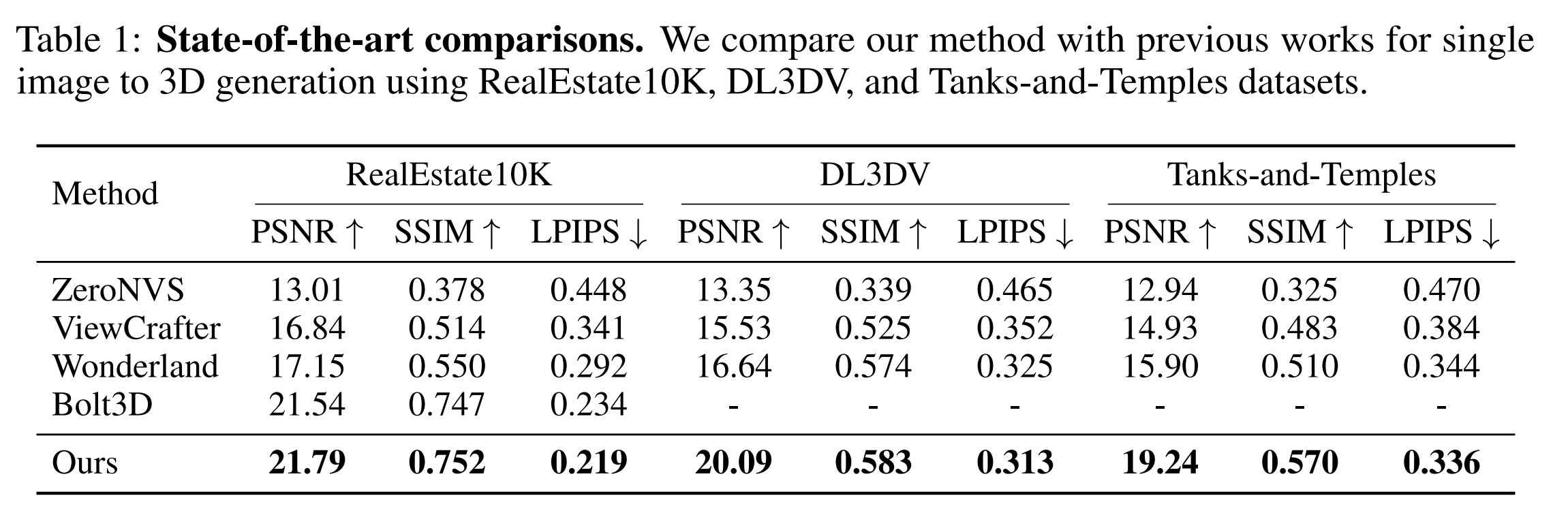
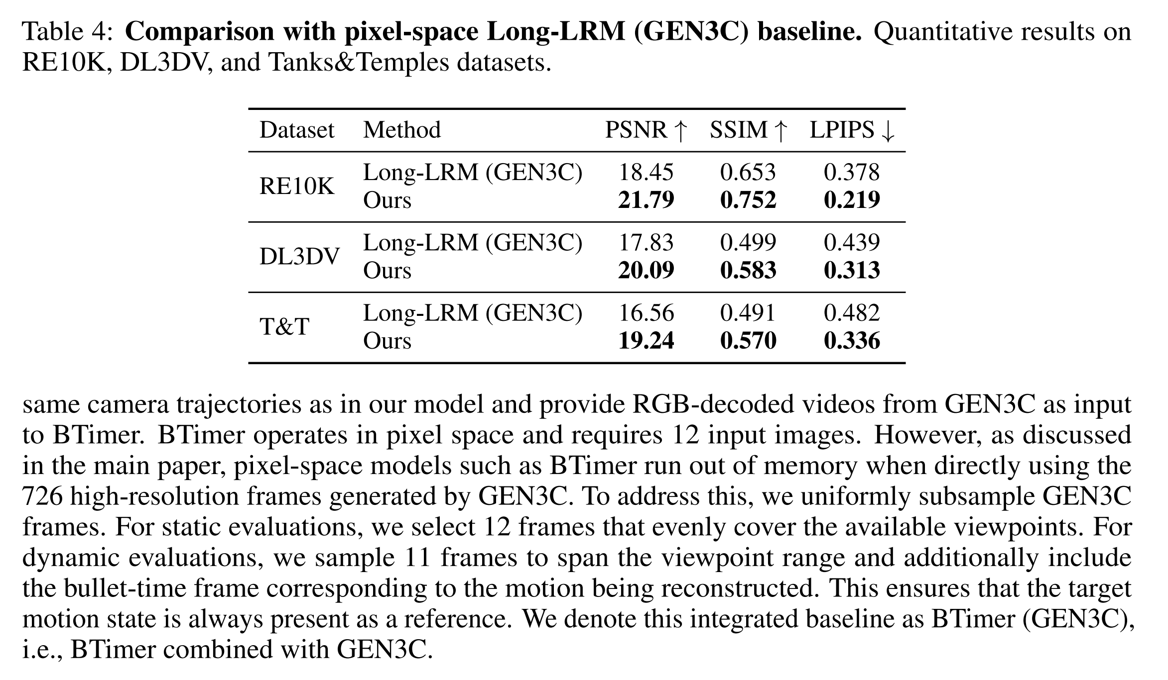
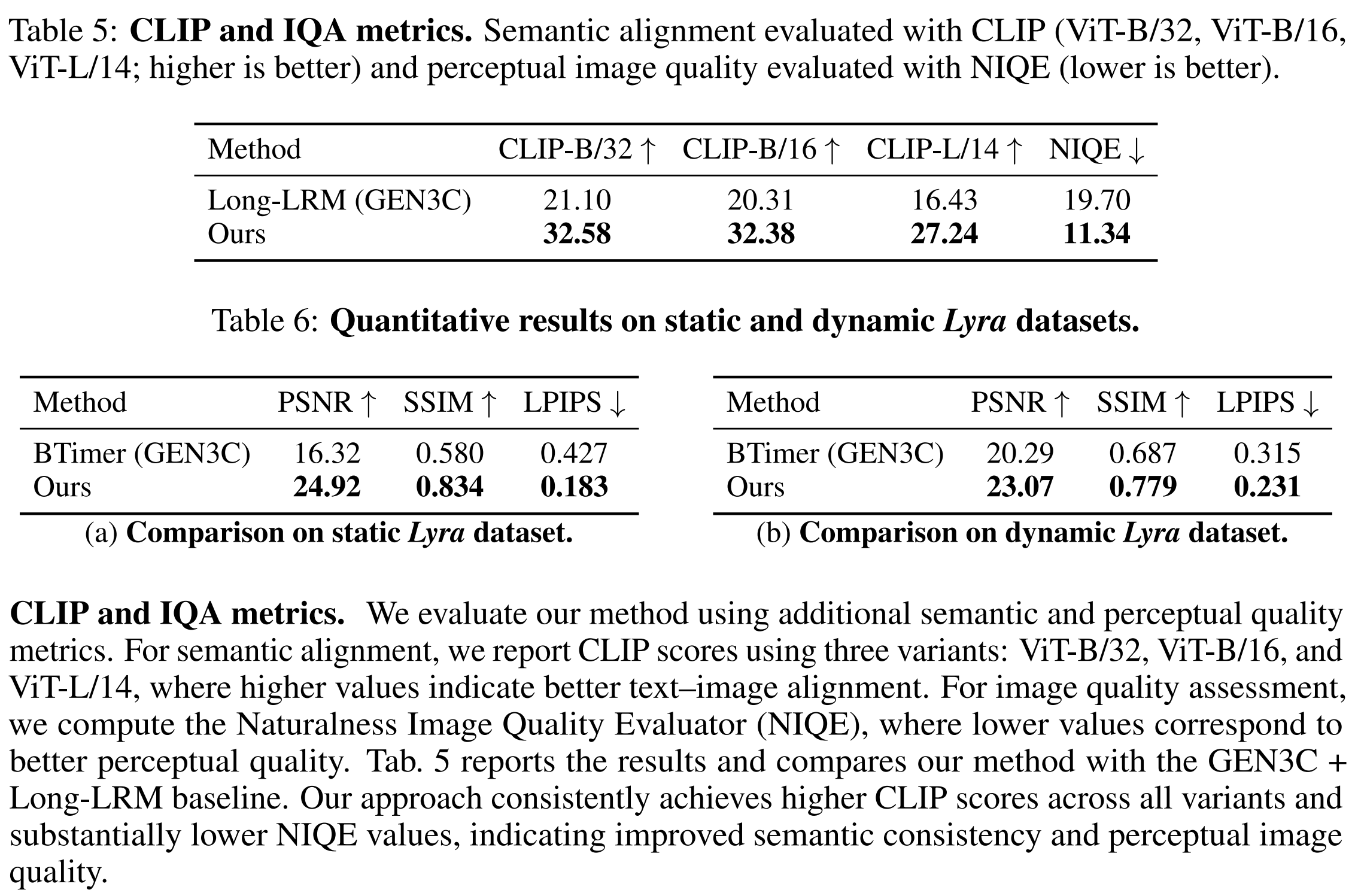
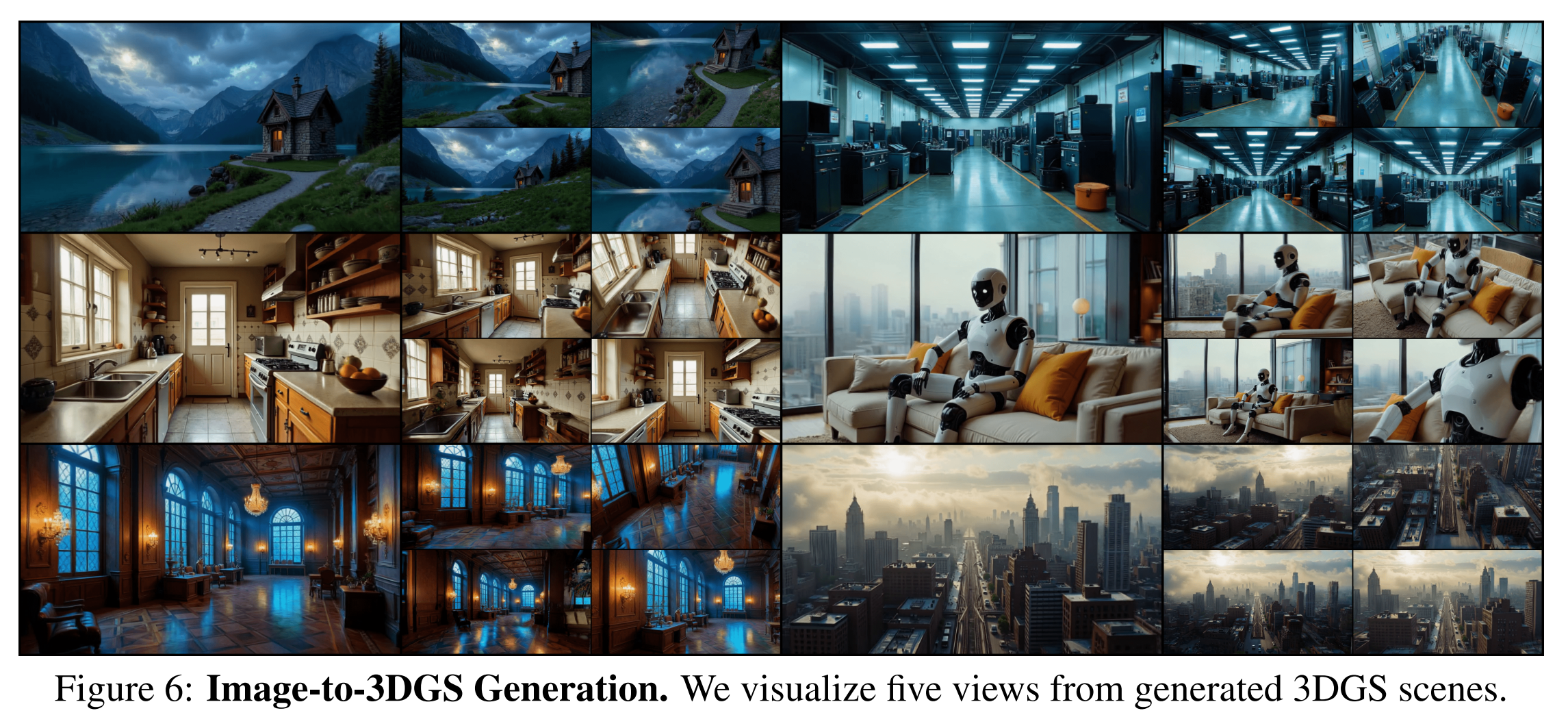
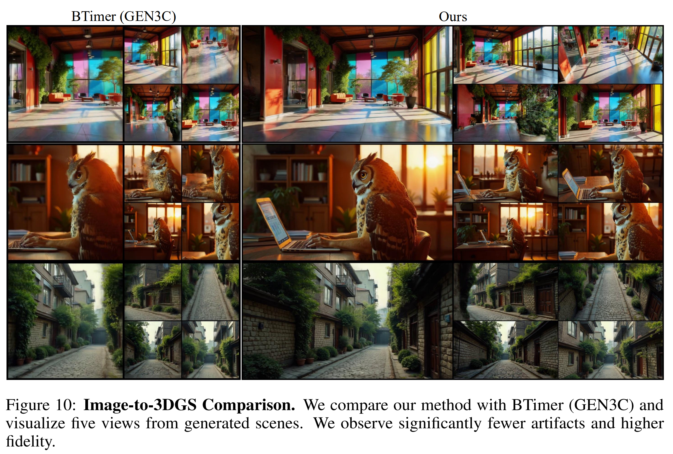
Lyra conducts an extensive set of experiments. It achieves the best PSNR, SSIM, and LPIPS performance across all three benchmarks. The qualitative results also show that, when the generated 3DGS is rendered from multiple novel viewpoints, it can synthesize regions that were not visible in the input while maintaining consistency with the input image.

The authors also argue that

improvements in the teacher video generation model can improve Lyra’s reconstruction quality as well, not just improvements to the reconstruction network itself.

This is how the authors interpret the results.

Ablation Study

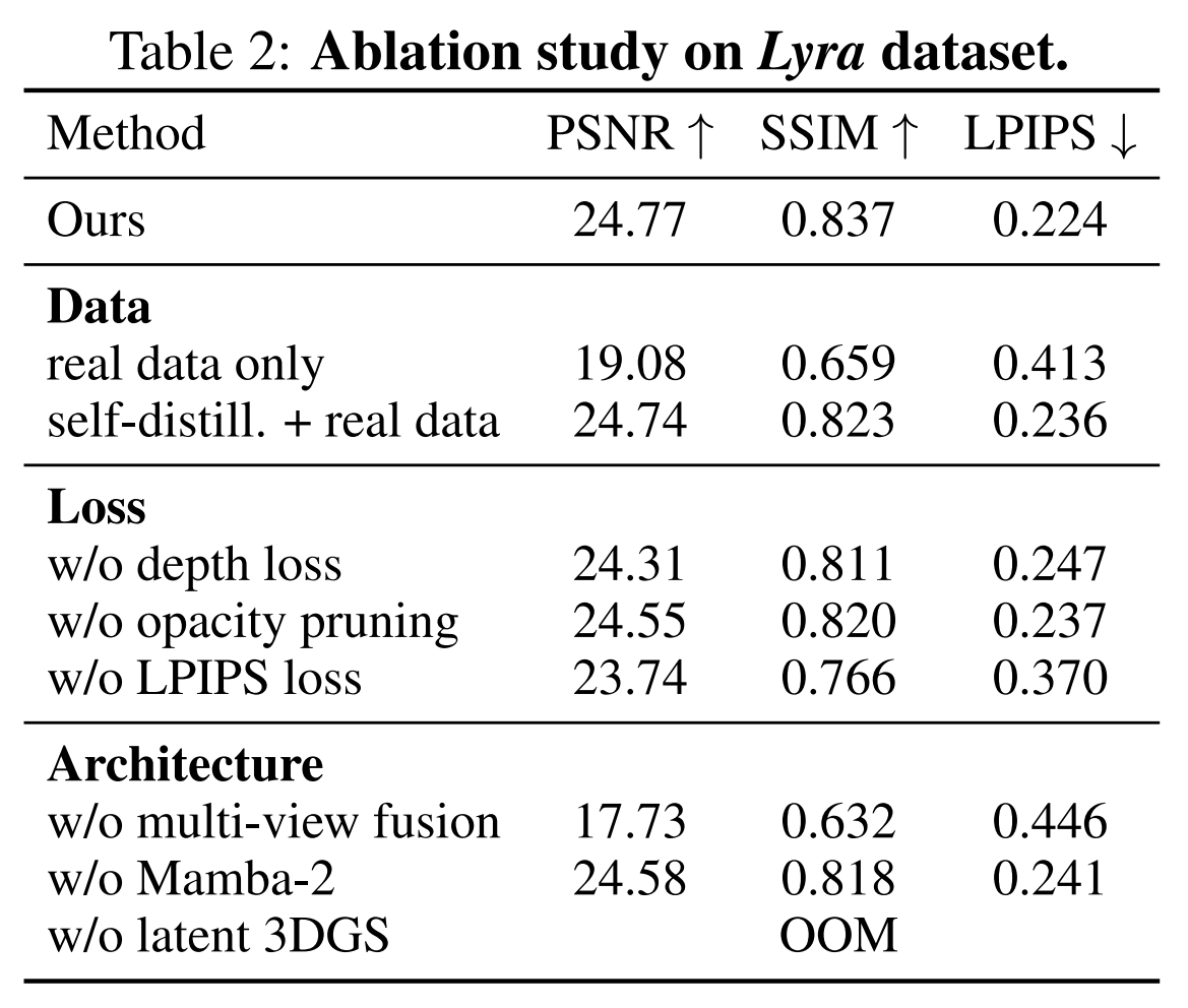
First, to verify the necessity of self-distillation, the table above shows that performance drops when the model is trained only on multi-view data (RealEstate 10K, DL3DV). In other words, the authors’ claim is that

synthetic supervision generated by video diffusion provides much more diverse scenes than real multi-view datasets, which is advantageous for OOD generalization.

Interestingly, combining self-distillation with real data still does not outperform the full model. The authors interpret this as evidence that synthetic self-distillation supervision is already sufficiently diverse and consistent on its own.

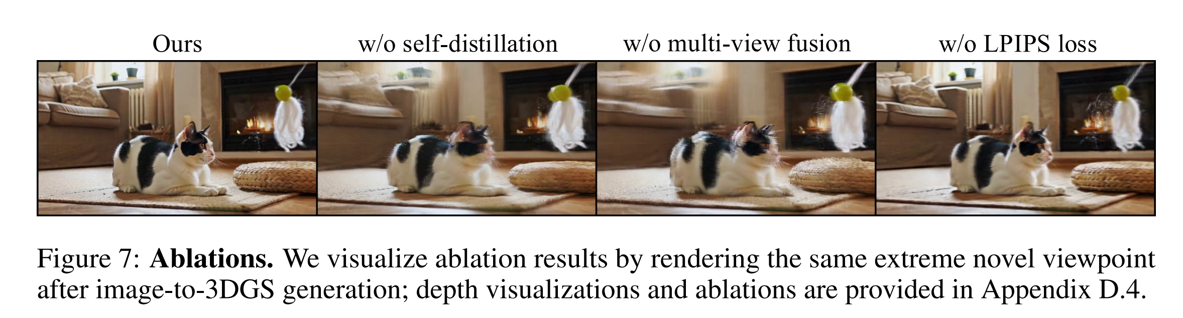
For the loss ablations, removing the depth loss causes the geometry to become flat, while removing the LPIPS loss substantially degrades performance. The paper explains that LPIPS improves robustness to input inconsistencies and helps preserve high-frequency details.

Removing opacity pruning also slightly reduces quality, and in particular, the comparison shows that pruning reduces rendering time.

On the architecture side, multi-view fusion appears to play an important role. Rather than independently generating Gaussians for each trajectory and merging the point clouds only at the end, the results show that it is important to fuse information from multiple trajectories already at the latent stage.

Removing Mamba-2 and using Transformer-only blocks does not greatly reduce quality, but it makes inference much slower. In addition, attempting 3DGS reconstruction in pixel space results in OOM because the number of input frames is too large.

Lyra includes many additional experiments, so the appendix is also worth referring to.

Contributions

1. It establishes a self-distillation framework that can be trained without a multi-view dataset.
2. It builds a framework that can be extended to dynamic scenes.
3. It achieves SOTA results across diverse scenes for single-image to 3D scene generation and single-video to 4D scene generation.

Limitations & Future works

The scale and geometric consistency of the 3D and 4D scenes synthesized by Lyra are directly bounded by the capacity of the camera-controlled video diffusion model that serves as the underlying Teacher. In other words, the quality and capability of the overall generation pipeline are fundamentally limited by the strength of the backbone video diffusion model.

The paper identifies the following directions for future work:

• integrating stronger video diffusion models into the framework
• investigating how auto-regressive techniques can be incorporated and adapted to the framework
• directly modeling motion and frame-tracking information more precisely within the reconstruction network

These are explicitly stated as future directions.