[Paper Review, EN] FlashWorld: High-Quality 3D Scene Generation within Seconds

Paper Information
Title: FlashWorld: High-Quality 3D Scene Generation within Seconds
Authors: Xinyang Li, Tengfei Wang, Zixiao Gu, Shengchuan Zhang, Chunchao Guo, Liujuan Cao
Venue: ICLR 2026 Oral
Link: [Paper], [Project], [Github]

Teaser Image (Poster)

Introduction

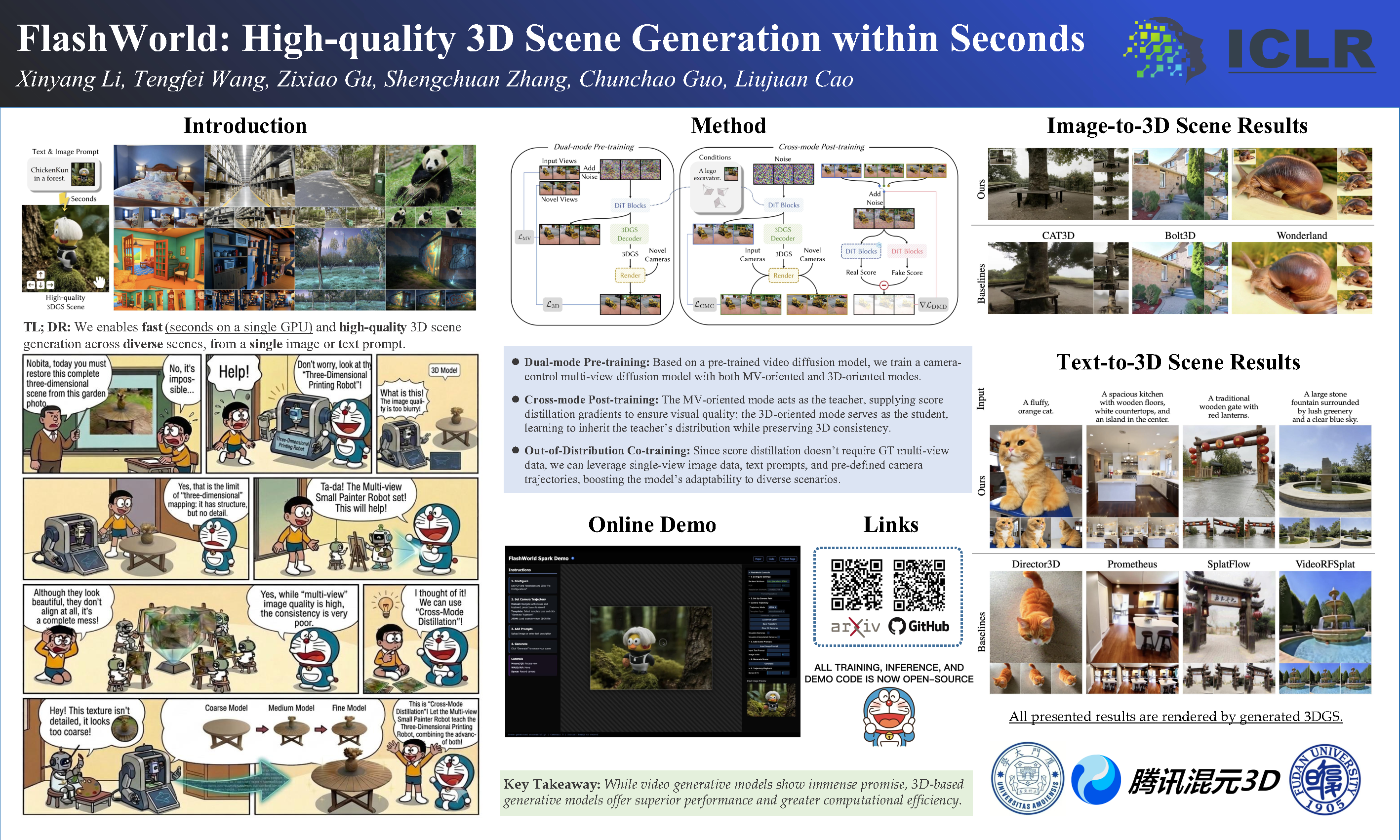
The field of 3D generation has grown rapidly, but the paper argues that it still faces two major obstacles: scarcity of high-quality 3D scene data and the exponential complexity of modeling real-world scenes.

There are two main paradigms for addressing this problem.

The first is the multi-view-oriented (MV-oriented) pipeline. A diffusion model first generates images from multiple viewpoints based on a text prompt or a reference image, after which 3D reconstruction is performed. However, because there are no explicit 3D constraints during view synthesis, geometric or semantic inconsistencies can arise. In addition, the pipeline incurs considerable computational overhead and requires substantial generation time.

Post-training distillation techniques are often used to improve the efficiency of diffusion models. However, directly applying these distillation methods can amplify the inherent limitations of the underlying framework.

The second is the 3D-oriented paradigm. This approach combines a diffusion model with differentiable rendering. It can maintain geometric and physical consistency across objects and backgrounds, but the resulting visual quality tends to be somewhat blurry. Moreover, it often requires an additional refinement stage.

Preliminary

To understand cross-mode post-training, which is the core of FlashWorld, it is first necessary to understand Diffusion Models and Distribution Matching Distillation (DMD).

Diffusion Model

A diffusion model typically starts from Gaussian noise and progressively removes the noise to generate samples from the target data distribution.

The forward process that adds Gaussian noise to the original data \(x\) according to timestep \(t\) is defined as follows:

\[x_t = F(x,t) = \alpha_t x + \sigma_t \epsilon, \qquad \epsilon \sim \mathcal{N}(0,I)\]

Here, \(\alpha_t\) and \(\sigma_t\) determine the ratio of signal to noise at timestep \(t\).

In other words,

\[x_t = \underbrace{\alpha_t x}_{\text{signal}} + \underbrace{\sigma_t\epsilon}_{\text{noise}}\]

which can be interpreted as the sum of the signal and noise components.

The denoising network takes the noisy sample \(x_t\) and timestep \(t\) as input and is trained to predict the original clean data \(x\).

\[\mathcal{L} = \mathbb{E}_{x,t,\epsilon} \left[ \left\| x-\hat{x}_\theta(x_t,t) \right\|^2 \right]\]

The equation above uses \(x\)-prediction, which directly predicts the clean data \(x\), but a diffusion model can also be trained to predict the noise \(\epsilon\) or \(v\), a linear combination of \(x\) and \(\epsilon\).

All of these predictions can be converted into a denoised estimate \(\mu(x_t,t)\), which allows the score of the distribution to be expressed as follows.

\[s(x_t,t) = \nabla_{x_t}\log p_t(x_t) = - \frac{x_t-\alpha_t\mu(x_t,t)} {\sigma_t^2}\]

Score

\[s(x_t,t)=\nabla_{x_t}\log p_t(x_t)\]

can be understood as a gradient indicating the direction in which the current sample \(x_t\) should move to reach a region of higher probability under the data distribution.

In other words, a diffusion model not only predicts a denoised result but can also provide a score field that indicates how the current sample should move toward the data distribution.

Distribution Matching Distillation (DMD)

Distribution Matching Distillation (DMD) is a method for distilling a diffusion model that requires many denoising steps into a generator that can perform generation in only a few steps.

Suppose a conventional diffusion teacher generates a sample through

\[z \rightarrow x_{T-1} \rightarrow x_{T-2} \rightarrow \cdots \rightarrow x_0\]

a long sequence of denoising steps. The goal of DMD is to match the distribution produced by the few-step student generator \(G_\theta\) to the target distribution represented by the teacher.

That is,

\[p_{\text{fake}} \rightarrow p_{\text{real}}\]

the student generator is trained so that this distributional matching occurs.

Here, \(p_{\text{real}}\) denotes the target distribution represented by the teacher diffusion model, while \(p_{\text{fake}}\) denotes the distribution currently produced by the student generator \(G_\theta\)

respectively.

In DMD, randomly sampled noise \(z\) is fed into the student generator to obtain

\[x_{\text{fake}} = G_\theta(z)\]

and noise corresponding to timestep \(t\) is then added again.

\[x_t = F(G_\theta(z),t)\]

For this noisy sample, the scores of the real and fake distributions are computed separately.

\[s_{\text{real}}(x_t,t) = \nabla_{x_t} \log p_{\text{real}}(x_t)\] \[s_{\text{fake}}(x_t,t) = \nabla_{x_t} \log p_{\text{fake}}(x_t)\]

The core DMD gradient uses the difference between these two scores as follows.

\[\nabla \mathcal{L}_{\mathrm{DMD}} = - \mathbb{E}_{t} \left[ \int \left( s_{\mathrm{real}} \left( F(G_\theta(z),t),t \right) - s_{\mathrm{fake}} \left( F(G_\theta(z),t),t \right) \right) \frac{dG_\theta(z)}{d\theta} \,dz \right]\]

The key term here is

\[s_{\text{real}} - s_{\text{fake}}\]

.

Using the definition of the score,

\[s_{\text{real}} - s_{\text{fake}} = \nabla_x\log p_{\text{real}}(x) - \nabla_x\log p_{\text{fake}}(x)\]

and therefore,

\[s_{\text{real}} - s_{\text{fake}} = \nabla_x \log \frac{p_{\text{real}}(x)} {p_{\text{fake}}(x)}\]

which can be interpreted as the gradient of the log-density ratio.

Therefore, \(s_{\text{real}}-s_{\text{fake}}\) is not merely used to propagate a loss to the student. It can be understood as a gradient indicating how the current output distribution of the student should be adjusted relative to the real distribution.

This signal is then propagated through

\[\frac{dG_\theta(z)}{d\theta}\]

to the generator parameters \(\theta\),

\[p_{\text{fake}} \rightarrow p_{\text{real}}\]

thereby training the student generator so that its distribution approaches the real distribution.

Real Score Model and Fake Score Model

In DMD, \(s_{\text{real}}\) and \(s_{\text{fake}}\) are not directly available, so each score is estimated using a diffusion model.

For the real score, a pretrained diffusion model

\[\mu_{\text{real}}\]

is used.

Because $\mu_{\text{real}}$ has already been trained on the target data distribution, it remains frozen during training.

In contrast, the fake distribution changes continuously as the student generator is trained.

\[p_{\text{fake}}^{(0)} \neq p_{\text{fake}}^{(1)} \neq p_{\text{fake}}^{(2)} \neq \cdots\]

Therefore, a separate diffusion model is required to estimate the score of the fake distribution:

\[\mu_{\text{fake}}\]

.

$\mu_{\text{fake}}$ is continuously updated using a diffusion loss on samples generated by the current student generator, so that it learns to estimate the current

\[p_{\text{fake}}\]

distribution.

The overall structure can be understood as follows.

\[z \rightarrow G_\theta(z) \rightarrow F(G_\theta(z),t)\]

The generated noisy sample is fed into both score models.

\[F(G_\theta(z),t) \rightarrow \begin{cases} \mu_{\text{real}} \rightarrow s_{\text{real}} \\ \mu_{\text{fake}} \rightarrow s_{\text{fake}} \end{cases}\]

Then,

\[s_{\text{real}}-s_{\text{fake}}\]

is used to update the student generator \(G_\theta\).

Why DMD Accelerates Inference

The main purpose of DMD is not to make training itself faster, but to reduce the number of denoising steps required at inference time.

Suppose a conventional multi-step diffusion teacher generates a sample from the target distribution through

\[z \xrightarrow{\text{many denoising steps}} x\]

. DMD instead trains the student so that

\[z \xrightarrow{\text{few steps}} \hat{x}\]

alone is sufficient to produce a sample satisfying

\[p(\hat{x}) \approx p(x)\]

.

In other words, the student does not reproduce the teacher’s long denoising trajectory itself. Instead, the few-step generator is trained to reproduce the output distribution that the teacher eventually forms through many denoising steps.

Therefore, distillation training still requires a real score model, a fake score model, and a student generator, so the training process itself is not necessarily simpler. Once training is complete, however, neither the teacher nor the fake score model is needed at inference time; only the few-step student is used.

In summary,

\[\boxed{ \text{DMD: Multi-step Teacher Distribution} \rightarrow \text{Few-step Student Generator} }\]

In FlashWorld, DMD is used to transfer the distribution of the MV-oriented mode, which has high visual quality, to a 3D-oriented few-step generator that possesses 3D consistency.

Method & Technical Details

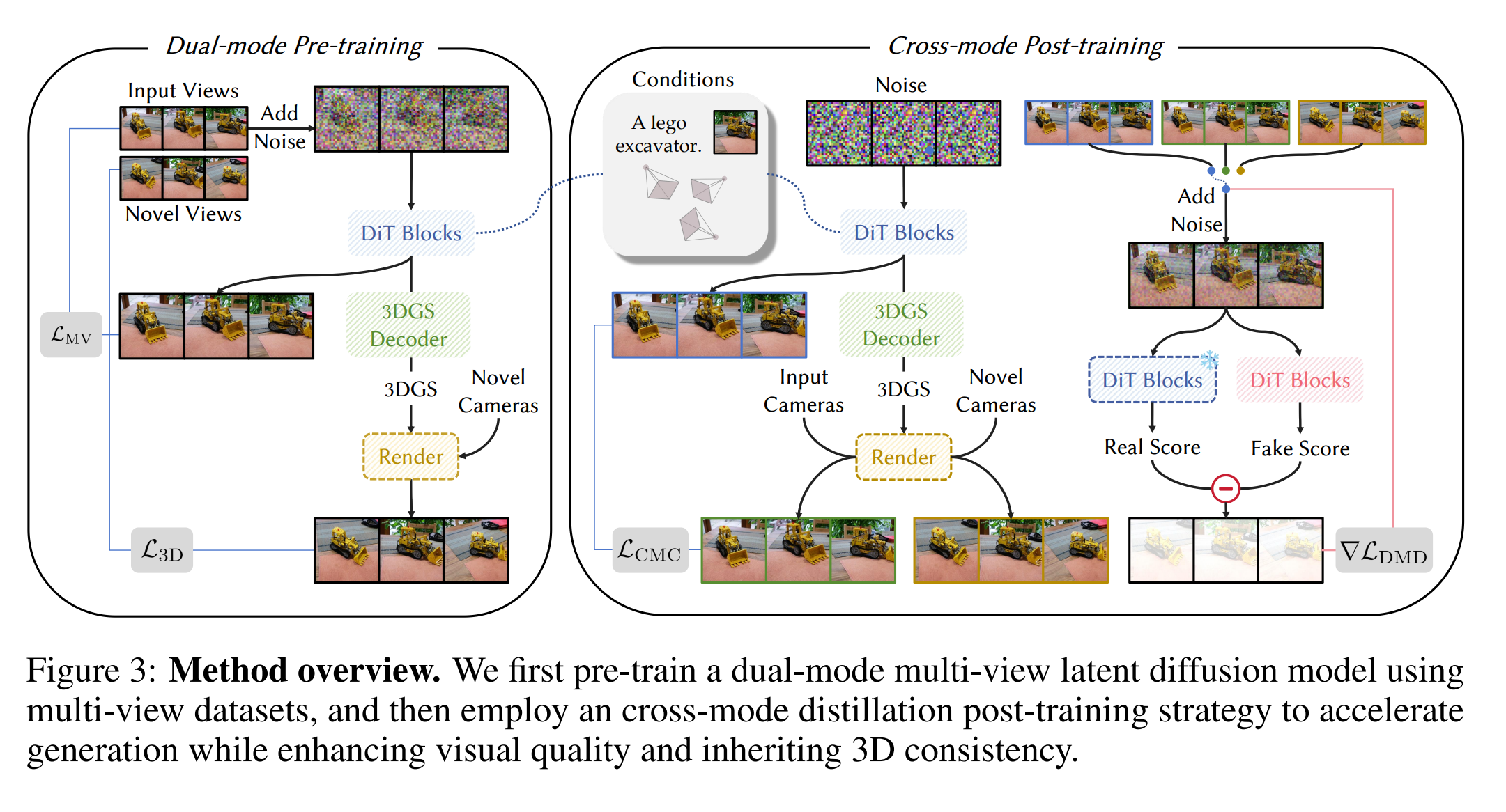
The goal of the method is to distill a well-trained “MV-oriented multi-view diffusion model” capable of generating high-quality multi-view images into a “3D-oriented generator” that provides 3D consistency in only a few steps, using the DMD technique described above.

To achieve this, the authors identify two challenges that must be addressed:

1. The 3D-oriented few-step generator needs a sufficiently robust prior and strong generative capacity.
2. Because high-quality multi-view datasets are limited, a strategy is needed to handle variables such as diverse styles, objects, and camera trajectories.

Dual-mode Pre-training

The authors first propose a framework that lays the foundation for addressing these challenges.

Here, dual-mode refers to the following two modes:

1. MV-oriented mode: predicts multi-view images
2. 3D-oriented mode: directly constructs 3DGS from intermediate features and renders it

First, multi-view images $X = {X_1, X_2, … , X_V}$ are sampled from the training dataset. The corresponding camera parameters for each view, $C={C_1, C_2, … , C_V}$, are also obtained. In addition, a condition $y$ such as a text prompt or a single-view image is provided.

Once these inputs are prepared,

\[Z = E(X)\]

the input multi-view images $X$ are passed through the VAE encoder $E$ and converted into latent representations. This produces a set of latents for a batch of multi-view data as follows:

\[Z = \{Z_1, Z_2, Z_2, ...\}\]

Next, as in standard diffusion training, a random timestep $t$ is sampled and noise is added.

\[Z_t = \alpha Z + \sigma_t \epsilon\]

As expected, the model now operates on the noisy multi-view latent $Z_t$ rather than directly on the input multi-view images used for training. The final inputs to the denoising network are therefore:

\[(Z_t, C, y) \rightarrow \text{Denoising Network}\]

These correspond, in order, to the noisy latent, camera parameters, and condition. The camera parameters are represented using a Reference-Point Plücker Coordinates raymap, a commonly used representation for camera parameters in multi-view 3D generation.

The denoising network is based on a Diffusion Transformer (DiT) with additional 3D attention blocks. The network outputs two quantities:

\[\hat{Z}_{MV}, F\]

These are, respectively, the clean multi-view latent for the MV-oriented mode and an auxiliary feature containing multi-view scene information. The latter is subsequently passed to a 3DGS decoder to construct 3D Gaussians for the 3D-oriented mode. In other words, the pipeline splits into two branches from this point onward.

For the MV-oriented mode, the DiT takes $Z_t, C, y$ as input and predicts $\hat{Z}_{MV}$. This prediction is then compared with the ground-truth clean latent $Z$:

\[\mathcal{L}_{MV} = \mathbb{E}_{X, t, \epsilon, y, C} [\lVert Z - \hat{Z}_{MV} \rVert ^ 2]\]

This is a diffusion objective that learns to convert a noisy multi-view latent into a clean multi-view latent. Importantly, the MV-oriented mode does not directly produce a 3D representation. Instead, it directly generates an image corresponding to each camera view. Because each view is independently generated by diffusion in image space, there is no guarantee that view 1 and view 2 originate from the same 3D geometry.

In other words, pure diffusion can produce high-quality outputs due to its strong generative capability, but it can suffer from multi-view inconsistency.

To address this problem, the second branch, the 3D-oriented mode, is introduced. The intermediate/output feature $F$ from the DiT is passed into a separate 3DGS decoder $D_G$:

\[D_G(F) = \{\tau, q, s, \alpha, c\}\]

The decoder outputs depth, rotation quaternion, scale, opacity, and spherical harmonics coefficients, respectively. More simply, it predicts parameters related to depth, rotation, size, opacity, and color, which together define the 3D Gaussian parameters.

Anyone familiar with 3DGS will notice that standard 3DGS primitives normally include the Gaussian position $\mu$. However, the parameters above do not contain an explicit position parameter; instead, they contain depth $\tau$. Rather than predicting the position directly, the authors use this depth value to obtain the position:

\[\mu = o + \tau d\]

Here, $o$ is the camera origin, $d$ is the ray direction, and $\tau$ is the predicted depth. Conceptually, this operation is performed at the pixel level, lifting a 3D Gaussian corresponding to each pixel.

This completes the final set of Gaussian parameters:

\[G = \{\mu, q, s, \alpha, c\}\]

The 3DGS renderer $R$ can then be used to render the scene from a novel camera view:

\[R(G, C_{novel})\]

The next question is what objective should be used. In practice, obtaining ground-truth values for 3D Gaussian parameters is difficult. Different depth estimation models can predict different depth values for the same pixels, which would in turn place the Gaussians at different positions. Ultimately, if a generated scene appears geometrically plausible as a 3D scene to the viewer, it can be regarded as a valid result. In other words, there is no direct ground truth for these parameters:

\[\mu_{GT}, q_{GT}, s_{GT}\]

For this reason, most 3D generation papers use rendering supervision, comparing a rendering of the scene from a particular view against the corresponding target image:

\[\mathcal{L}_{3D} = \mathbb{E} [\lVert X_{novel} - R(G, C_{novel}) \rVert ^2]\]

A notable difference here is that many conventional methods determine a fixed set of camera views (pose 1 to pose n) before running the pipeline and perform supervision only on those views, whereas this paper takes a different approach.

The scene is rendered from novel views, and supervision is also applied to those novel views.

The reason is that if reconstruction loss is applied only to the input views, the scene may look correct from those views while having an incorrect 3D structure from other viewpoints. By applying novel-view reconstruction loss so that the scene must also appear correct from viewpoints outside the input views, the Gaussians must be arranged consistently across multiple viewpoints, creating a 3D consistency constraint. As a result, the model obtains 3D-consistent rendered multi-view images at the camera views $C$ defined by the training dataset.

The MV-oriented branch ultimately produces the clean multi-view latent $\hat{Z}_{MV}$. Similarly, the 3D-oriented branch produces $\hat{Z}_{3D}$. This is simply the latent obtained by passing the rendered multi-view images through the VAE encoder $E$:

\[\hat{Z}_{3D} = E(R(G, C))\]

cross-mode post-training

Next, the paper trains the model through distillation so that it can generate a 3D scene in only a few steps.

In the preliminary section, we saw that DMD involves

\[\mu_{real}, \mu_{fake}, G_{\theta}\]

In this pipeline, these can be understood, respectively, as the MV-oriented mode serving as the teacher, a model that estimates the fake score of the 3D student distribution, and the 3D-oriented few-step generator serving as the student.

Here, $\mu_{real}$ is kept frozen. Although the 3D-oriented mode previously used many steps, the method does not simply run that same many-step process here. Instead, the previously trained 3D-oriented mode is used to initialize the current few-step student. In other words, no entirely new architecture is added on top of the architecture introduced in the dual-mode pre-training section.

The method largely inherits the 3D-oriented pipeline from the previous section:

\[(\{Z_{t_i}, t_i, y, C\} \rightarrow DiT \rightarrow F_i \rightarrow D_G \rightarrow G_i) \rightarrow R(G_i,C) \rightarrow E(R(G_i,C)) \rightarrow \text{noise injection} \rightarrow Z_{t_{i+1}}\]

Here, the pipeline inside the parentheses can be regarded as one denoising step of the 3D-oriented generation process, $G_{\theta, 3D}$, and the goal is to complete the generation in only four such steps. It is important not to confuse this with the DiT having only four timesteps; rather, the entire process is executed four times. The paper uses the timestep schedule $t_i={1000, 900, 759, 500}$. At the end of each step, noise injection is performed and the resulting latent is passed to the next step $t_{i+1}$.

With this pipeline defined, the method applies DMD2. The original 3D-oriented branch used many steps, so directly replacing it with a four-step branch would not guarantee output quality. Therefore, the few-step student must be trained again so that it can reach a high-quality output distribution even with only a few steps.

The frozen model $\mu_{real}$ is used as the teacher to estimate $s_{real}$, the score of the high-quality MV distribution. Meanwhile, $\mu_{fake}$ continuously tracks the student $G_{\theta, 3D}$ and estimates $s_{fake}$, the score of the student-generated distribution $p_{fake}$. Because $p_{fake}$ changes whenever the student is updated, $\mu_{fake}$ must also be continuously updated.

That is,

\[s_{MV} - s_{\text{current 3D student}} = s_{real} - s_{fake}\]

This gradient is used to update $G_{\theta, 3D}$, so that

\[p_{\text{3D student}} \rightarrow p_{MV}\]

the student distribution approaches the MV distribution. In addition, the DMD2 loss combines the DMD loss with a GAN loss:

\[L_{DMD2} \approx L_{DMD}+\lambda_{GAN}L_{GAN}\]

Here, $\lambda$ is the R1 regularization term. Conceptually, the discriminator is trained so that

\[D(X_{real}) \rightarrow 1 D(X_{fake}) \rightarrow 0\]

while the generator $G_{\theta, 3D}$ is trained so that

\[D(X_{fake}) \rightarrow 1\]

.

However, this raises a concern: the 3D student may eventually lose its strength in 3D consistency and be pulled toward the MV-oriented distribution. Of course, because the 3D-oriented branch renders from a single shared 3D scene, it may appear that updates through this gradient naturally preserve 3D consistency.

The authors argue that 3D consistency is maintained for the following three reasons, but I do not think these arguments alone are sufficient to demonstrate it conclusively:

1. 3D supervision (rendering supervision on novel views, as described in the previous section)
2. Initialization from pretrained 3D-oriented weights
3. Repeatedly performing $G_i \rightarrow \text{Render}$ at every step

In my view, the second point is particularly important. Since these weights will continue to be updated toward the MV-oriented distribution, it is unclear how the model avoids losing its advantage in 3D consistency. This is because the MV side remains fixed while only the 3D side is updated.

The authors additionally introduce a Cross-Mode Consistency Loss. For this, they use an MV-oriented student branch that shares the DiT backbone used by the 3D student.

\[\begin{aligned} \hat{Z}_{3D} &= E(R(G_{\theta, 3D}(Z_t, t_i, y, C), C)) \\ \hat{Z}_{MV} &= G_{\theta, MV}(Z_t, t_i, y, C) \end{aligned}\]

Using these predictions,

\[\mathcal{L}_{CMC} = \lVert \hat{Z}_{3D} - \hat{Z}_{MV} \rVert ^2\]

the two outputs are matched with this loss. This is an auxiliary loss intended to reduce floating artifacts and unstable 3D predictions that arise during DMD2. The MV-oriented student is also updated at a lower frequency, and the predictions of the two modes are aligned.

In summary, the 3D student receives the following signals:

\[\underbrace{\mathcal{L}_{\mathrm{DMD}}}_{\text{move toward the MV teacher distribution}} + \underbrace{\mathcal{L}_{\mathrm{GAN}}}_{\text{make the rendering real/high-quality}} + \underbrace{\lambda \mathcal{L}_{\mathrm{CMC}}}_{\text{stabilize the 3D branch}}\]

Out-of-Distribution Data Co-Training

This training setup introduces another minor issue. FlashWorld is trained on MVImgNet, RealEstate10K, and DL3DV10K. The DiT backbone, however, has also been exposed to large-scale image and video data beyond these three multi-view datasets, so it can robustly handle inputs outside their distribution. In contrast, the 3DGS decoder in the 3D branch has only been trained on these three multi-view datasets and is therefore less robust to other types of data.

In other words, the 3DGS decoder $D_G$ has only experienced the multi-view distribution.

A natural solution is therefore to broaden the input distribution seen by the 3DGS decoder. To do this, the pipeline is additionally trained using only a single image or text as the initial condition rather than multi-view data.

When only text or a single-image condition $y$ is provided, a camera trajectory $C$ is supplied together with it and the model is trained using only the DMD-based objectives. Because no real ground truth is available, the GAN loss is omitted, and training uses only the DMD and CMC losses:

\[(y, C_{random}) \rightarrow DiT \rightarrow F \rightarrow D_G \rightarrow G\]

The camera trajectories are drawn from existing multi-view datasets such as RealEstate10K and WorldScore. This co-training is performed during the post-training stage, not pre-training, and mixes multi-view data and OOD data at a 2:1 ratio.

Experiments

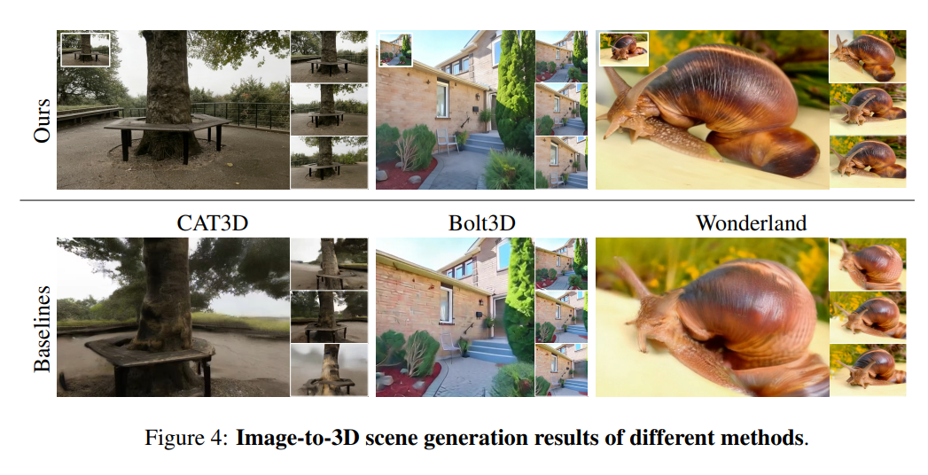
Figure 4 compares FlashWorld against MV-oriented baselines and highlights the strengths of its 3D-oriented pipeline. Although the baseline methods are not open-sourced, the authors use the video results provided on their project pages and employ ViPE to estimate camera poses and intrinsics, allowing the results to be rendered from angles that are as similar as possible.

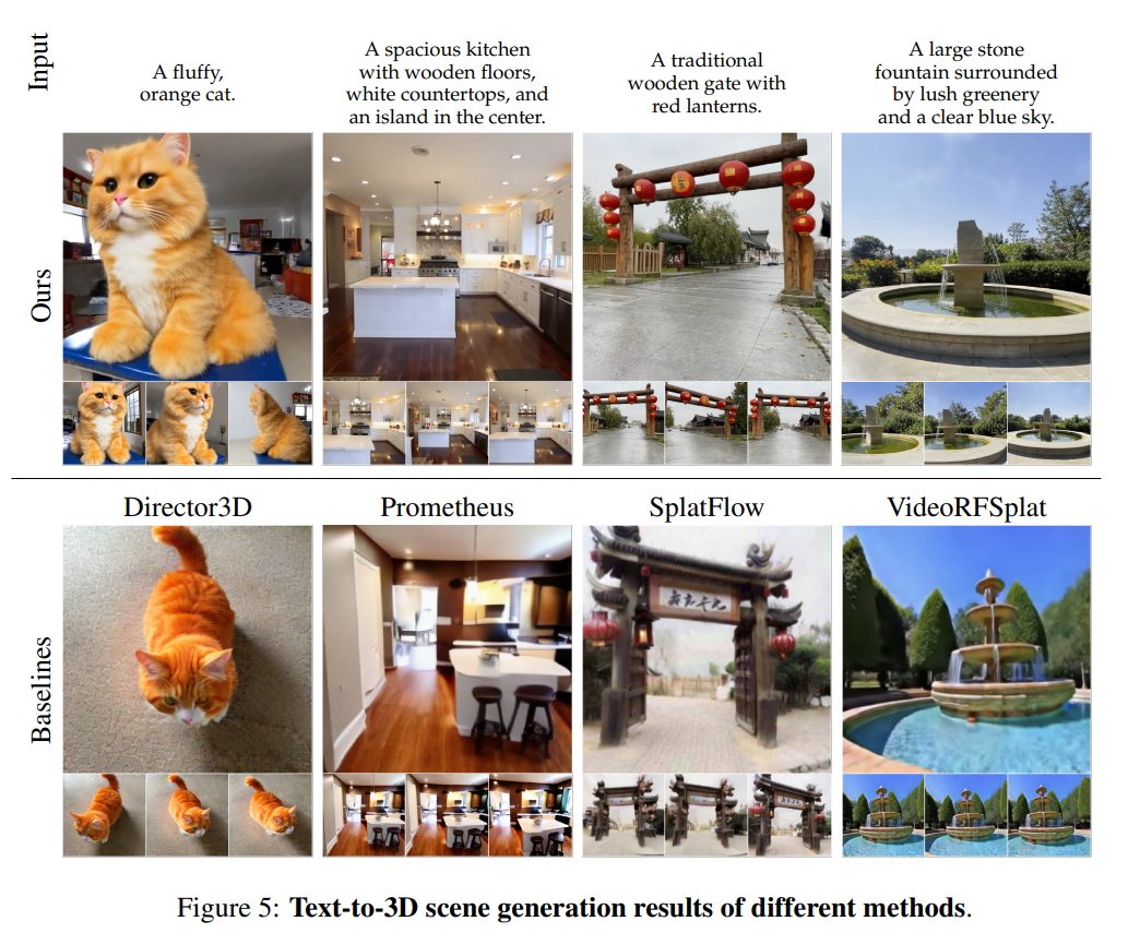
For text-based generation, both qualitative and quantitative comparisons are conducted. In the qualitative evaluation, Prometheus often produces blurry scenes and incorrect geometry because of the inherent inconsistency of the MV-oriented pipeline. SplatFlow and VideoRFSplat likewise suffer from blurry artifacts and have difficulty reproducing fine details such as those found in floors and grass.

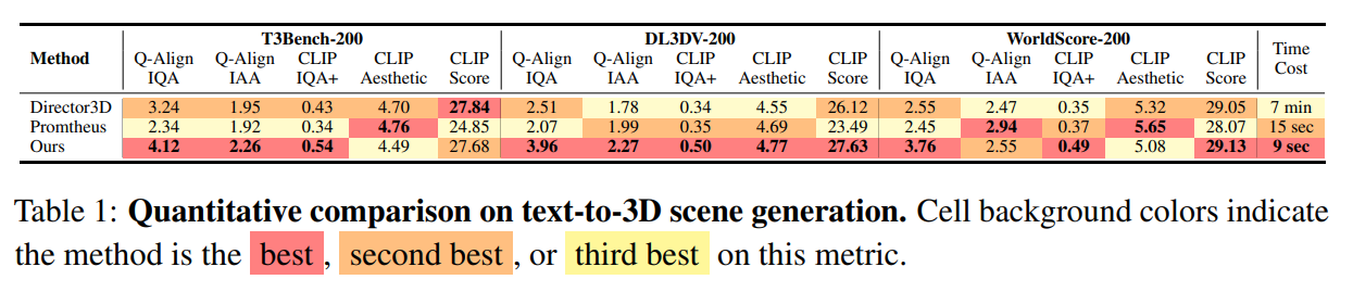
For the quantitative evaluation, 600 text prompts are sampled from T3Bench, DL3DV, and WorldScore. Because all compared methods in this table are based on 3D Gaussian representations, metrics related to camera control and 3D consistency are not applicable in this experimental setting. The evaluation therefore focuses on quality metrics including CLIP IQA+, CLIP Aesthetic, CLIP Score, and Q-Align. In particular, CLIP-Aesthetic sometimes tends to favor smooth outputs, which may not always align with the detailed and realistic results produced by this method.

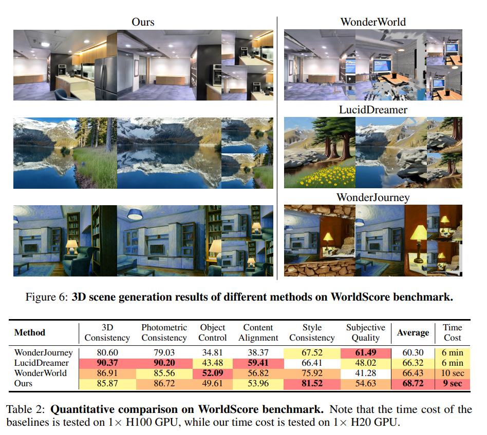
The authors also evaluate FlashWorld on the WorldScore benchmark, comparing it against the 3D generation methods WonderJourney, LucidDreamer, and WonderWorld. Because the comparison focuses exclusively on 3D generation methods, the Camera Control metric mainly reflects the robustness of each method to the evaluation protocol and is therefore considered less informative in this setting, so the authors omit it. In addition, the original WorldScore benchmark evaluates most metrics only on anchor frames, which can be suboptimal for 3D world generation tasks that require novel-view synthesis.

For a fairer comparison, the authors therefore re-evaluate the metrics on frames randomly sampled within specific intervals. FlashWorld achieves the highest average score and the fastest inference speed among all compared approaches.

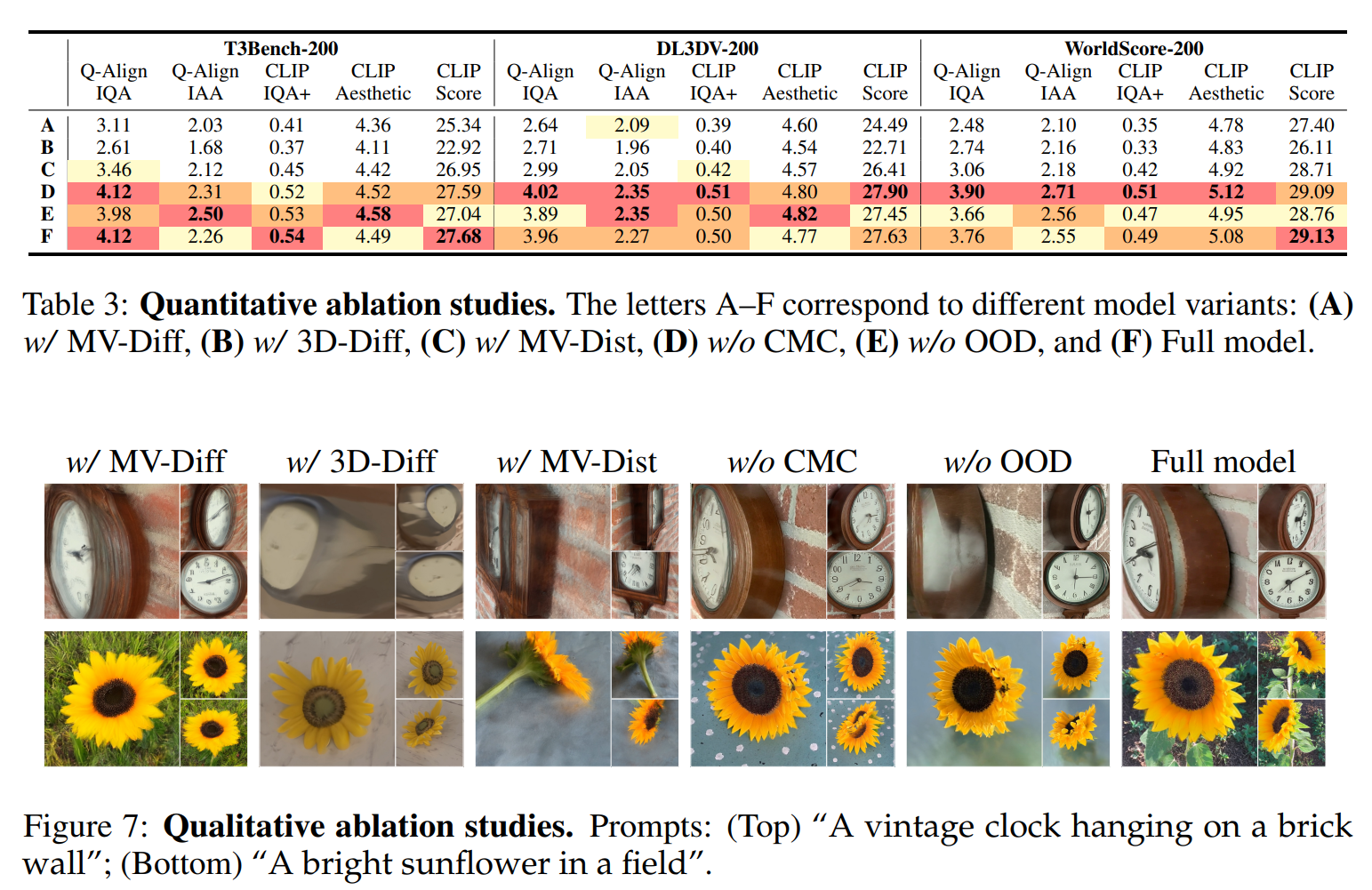
The authors also conduct various ablation studies. w/ MV-Diff denotes the MV-oriented diffusion model, w/ 3D-Diff denotes the 3D-oriented diffusion model, w/ MV-Dist denotes the MV-oriented model distilled into a few-step model, w/o CMC denotes the 3D-oriented model distilled into a few-step model without the CMC loss, and w/o OOD denotes the full cross-mode model without OOD co-training.

Interestingly, w/o CMC achieves better values than the full model on many metrics. This seems to suggest that, beyond the concern mentioned earlier that the 3D student may forget the distribution responsible for 3D consistency, the effectiveness of CMC itself is difficult to establish from the quantitative results alone.

Contributions

1. Introduces a pre-training strategy for training a multi-view diffusion model that operates in both MV-oriented and 3D-oriented modes.
2. Proposes a cross-mode post-training strategy that demonstrates robust performance in both visual quality and 3D consistency.
3. Introduces a novel strategy that improves generalization ability on out-of-distribution inputs.

Limitations & Future works

Even though the number of views is increased, the diversity and scale of the generated 3D scenes are still limited by the coverage of existing datasets. The model also has limitations in representing fine geometric structures, mirror reflections, and text. The authors suggest incorporating autoregressive generation and extending the framework to dynamic 4D scene generation as future research directions.

The following is an additional limitation identified by the reviewer:

It has not been demonstrated that the distilled student model can preserve the 3D-consistency distribution.