[Paper Review, EN] SeeU: Seeing the Unseen World via 4D Dynamics-aware Generation

Paper Information
Title: SeeU: Seeing the Unseen World via 4D Dynamics-aware Generation
Authors: Yu Yuan, Tharindu Wickremasinghe, Zeeshan Nadir, Xijun Wang, Yiheng Chi, Stanley H. Chan
Venue: CVPR 2026
Link: [Paper], [Project], [GitHub]

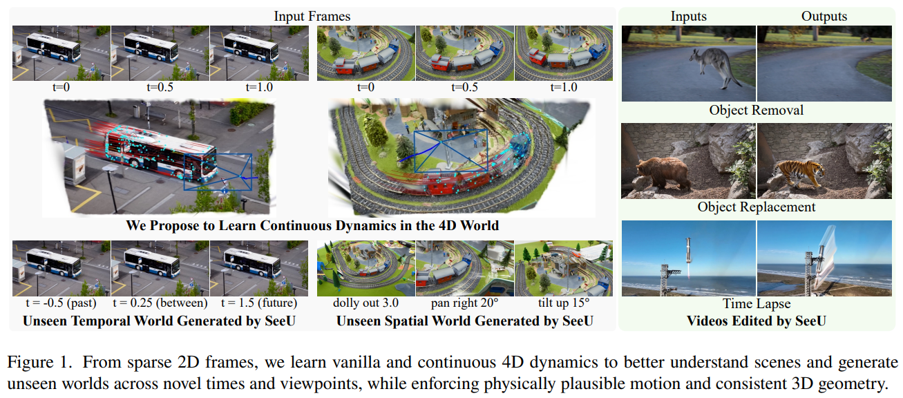
Teaser Image

Introduction

“Images and videos are 2D projections of the real world (4D).” This is how the authors of the paper describe them.

Many recent studies learn dynamics through a low-dimensional latent space, which improves computational efficiency. However, this approach has limitations:

1. Converting the information in 4D itself into 2D leads to the loss of crucial 3D structural information.
2. Changes in camera pose increase the complexity of scene motion.

As a result, because these models learn only 2D visual patterns without 3D or physical supervision, it is difficult for them to represent or understand 3D geometry and physical dynamics.

Therefore, the authors of SeeU design the overall pipeline around the 2D \(\rightarrow\) 4D \(\rightarrow\) 2D scheme to handle 4D dynamics and perform visual generation.

Method & Technical Details

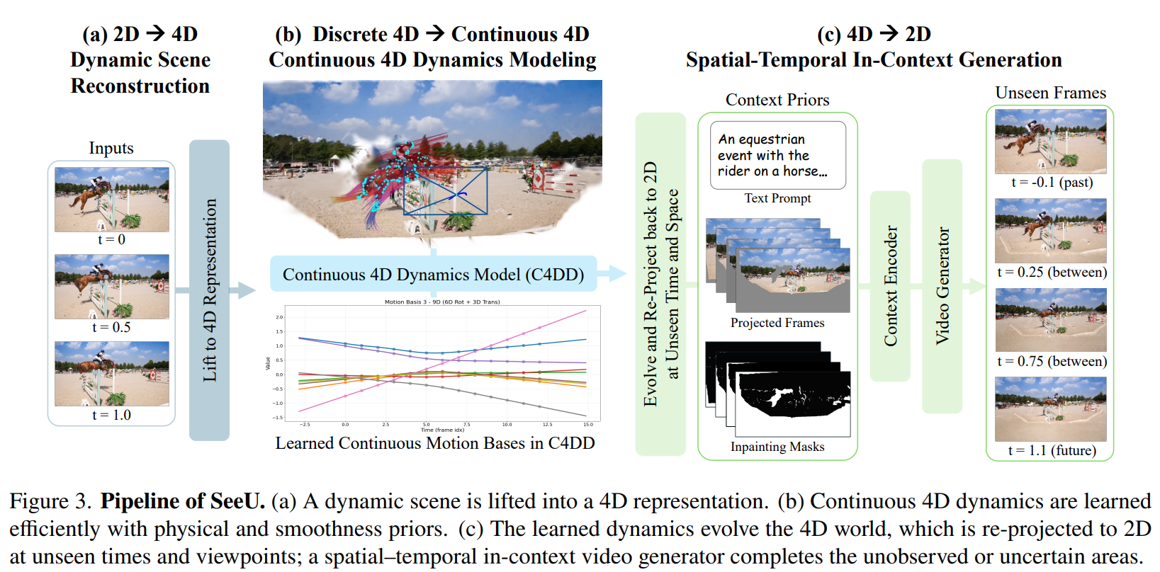
At a high level, the figure shows that the pipeline proceeds through (i) 2D \(\rightarrow\) 4D, (ii) Discrete 4D \(\rightarrow\) Continuous 4D, (iii) 4D \(\rightarrow\) 2D. I will explain each part in more detail below.

First, let us look at the input:

\[\{I_t \in \mathbb{R}^{H \times W \times 3}\}\]

This means that the method uses a monocular frame sequence of a dynamic scene.

1st stage: 2D \(\rightarrow\) 4D

Shape-of-Motion(Essential Concept)

The authors of this paper adopt and use an existing method from the ICCV 2025 paper “Shape of Motion: 4D Reconstruction from a Single Video.” They give the following reasons:

1. it can operate even with limited camera parallax, and
2. it can separate static regions from trackable dynamic elements.

These are the reasons given in the paper.

Earlier, when discussing the overview figure, I mentioned that the 2D \(\rightarrow\) 4D dynamic scene reconstruction is performed first; this is the stage where the above method is used.

I will also make a separate post about the SoM paper later.

For now, to understand this paper, SoM can be described as “a 4D reconstruction method that recovers not only camera motion but also the 3D motion trajectories of objects within the scene from a monocular video.”

For a typical static 3D reconstruction method:

\[\text{3D point} = (x,y,z)\]

it is enough to recover a single point, but for a moving scene,

\[x_i(t) = (x_i(t), y_i(t), z_i(t))\]

we also need to represent how the 3D position changes over time.

Then, to explain how SeeU performs 4D reconstruction using this method,

\[I_0, I_1, ... , I_T\]

it takes multiple frames from a monocular video as input and uses a model called MegaSaM to obtain the camera intrinsics, camera extrinsics, and depth map for each frame. For each frame t,

\[C_t = (K, R_t, t_t)\]

and

\[D_t(u,v)\]

can be obtained. Here, u and v represent the pixel location in 2D coordinates.

With this information, \((u,v)\) can be lifted to the 3D position \((X,Y,Z)\). In other words, it can be back-projected. Next, a moving foreground mask is obtained using Track-Anything. This separates the static background from the dynamic foreground.

Most importantly, a model called TAPIR is used to track the same point across multiple frames.

Suppose we track a certain pixel,

\[p_0 = (320,320)\]

and in the next frame it is located at

\[p_1 = (330, 250)\]

then we can obtain a 2D trajectory. However, this is only 2D motion on the image plane. To obtain a 3D trajectory, the camera pose and depth information from earlier are used to convert the 2D trajectory into a 3D trajectory. Specifically,

\[(u_t, v_t, D_t(u_t, v_t))\]

can be used to back-project it into a 3D point.

\[p_t^{2D}\]

is converted into

\[X_t^{3D}\]

However, a scene may contain many Gaussians, and learning an independent motion trajectory \(T_i(t)\) for every Gaussian would be inefficient. Therefore, SoM introduces the concept of a motion basis. Instead of allowing thousands or tens of thousands of points to move independently, the points share motion bases so that similar transformations can be shared. In other words, you can think of points as forming groups that share a common motion structure.

SoM compresses the overall motion into a small number of motion bases. In SeeU, this is expressed as follows:

\[P_t^i = P_0^i + B(t)w_i\]

Here, \(P_t^i\) denotes the state of Gaussian i at time t. In other words, the equation represents the state of Gaussian i at a particular time t by adding the product of the shared motion basis and its weights to the initial state of Gaussian i. The weights determine how the shared motion bases are combined. This enables soft motion decomposition, allowing motions to be combined appropriately without requiring hard object assignments.

At this point, it is possible to roughly infer why the method is called Shape-Of-Motion. Even if a large number of points appear to move in complex ways, the underlying 3D motion is assumed to have a low-dimensional structure that can be explained by only a few motion bases.

That is the basic idea behind SoM. Next, I will explain how SeeU builds on it.

When SoM is applied, it basically produces a discrete motion state for each observed frame. For example, suppose a point at \(t=0, 1, 2, 3\) obtains

\[B_0, B_1, B_2, B_3\]

respectively.

However, we may also want to know the motion at arbitrary unseen times such as \(t = 1.37, -0.5, 5.2\). To address this, SeeU introduces a method called C4DD.

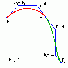
Whereas SoM produces discrete motion bases, C4DD converts them into a continuous B-spline like the one shown in the figure. A B-spline is a type of continuous function frequently used in computer graphics, so it is useful to be familiar with the concept.

Overall, SeeU can therefore be summarized as follows:

The motion bases are initialized from discrete 3D point trajectories using Procrustes analysis and refined with photometric reconstruction error (SoM); SeeU then converts them into continuous functions using B-splines.

The authors also represent the scene using a canonical 3D Gaussian set \(\{g_i^0\}_{i=1}^N\) that persists over time, parameterized as follows:

\[g_i^0 = (\mu_i^0, R_i^0, s_i, o_i, c_i)\]

Here, \(\mu\) denotes the canonical mean, \(R\) the canonical orientation, \(s\) the scale, \(o\) the opacity, and \(c\) the color. In order, these parameters can be understood as representing the Gaussian position mean, rotation, size, opacity, and color for a single Gaussian (these are essential parameters that repeatedly appear whenever 3D Gaussian Splatting is used in 3D or 4D vision, so I strongly recommend becoming familiar with them).

Now, the method must also represent how each Gaussian changes over the course of the frames. This is done through a per-frame rigid transformation:

\[T_{0 \rightarrow t} = [R_{0 \rightarrow t} , t_{0 \rightarrow t}] \in SE(3)\]

The change from frame 0 to frame t can be represented using rotation and translation matrices:

\[\mu_i^t = R_{0 \rightarrow t}\mu_i^0 + t_{0 \rightarrow t},\; R_i^t = R_{0 \rightarrow t}R_i^0\]

For the input frames, MegaSaM estimates the camera intrinsics, extrinsics, and per-frame depth; Track-Anything obtains masks for the dynamic foreground; and TAPIR extracts 2D point tracks. These are then used to output the frame-level camera pose and foreground Gaussian attributes \(P\).

2nd stage: Discrete 4D \(\rightarrow\) Continuous 4D

The next step is to convert Discrete 4D into Continuous 4D.

First, let us define two quantities. The camera pose and foreground Gaussian attributes obtained in Stage 1 are represented as follows:

\[C_t,\; P_t^i\]

The paper then points out two challenges:

1. Learning an individual 3D trajectory for each of the tens of thousands of Gaussians in a single scene is extremely inefficient.
2. The reconstructed trajectories should be smooth and physically plausible.

To solve the first challenge, the authors use the Shape-Of-Motion method explained earlier. Simply put, instead of injecting motion independently into each Gaussian, the Gaussians use a shared global motion basis. The paper refers to this approach as low-rank motion parameterization.

We can therefore represent the properties of a foreground Gaussian as follows:

\[P_t^i = P_0^i + \underbrace{B(t)}_{\in \mathbb{R}^{m \times K}} \underbrace{w_i}_{\in \mathbb{R}^{K}}, \;\;\;\; P_0^i,\; P_t^i \in \mathbb{R}^m\]

Here, \(B(t)\) is a set of global motion basis functions, and \(w_i\) is a time-invariant coefficient vector for Gaussian i. Instead of directly learning N separate trajectories, each Gaussian can be compactly represented using only a few coefficients over K shared basis functions \(B(t)\).

These discrete motion bases are initialized from 3D point trajectories using Procrustes analysis and are then progressively refined by minimizing the photometric reconstruction error (for a more detailed explanation of the SoM procedure, open the Shape Of Motion section above).

Through this first challenge, 3D trajectories can now be computed efficiently.

To solve the second challenge, the authors need a continuous representation. They call this method the Continuous 4D Dynamics Model (C4DD). The continuous function they use is a B-spline basis function:

\[\hat{B}_t = \sum_{j=1}^M N_{j,d} (t) q_j\]

Here, \(N_{j,d}\) is the B-spline basis function, and \(q_j\) is a learnable control point for the motion basis. The number of control points \(M\) controls the representational capacity of the curve. A larger \(M\) can capture richer temporal variations, whereas a smaller \(M\) provides stronger smoothness and regularization.

In the figure, you can see points associated with the blue curve. By moving the virtual points that control this curve, the shape of the corresponding part of the curve can be changed. Therefore, the number \(M\) described in the paper can be understood as the number of control points that determine the actual shape of the curve. This is a concept that appears frequently in computer graphics.

During training, the B-spline control points of the shared motion bases and the B-spline control points of the camera trajectory are optimized using the following objective function:

\[L_{total} = L_{data} + \lambda_{phys} L_{phys}\]

The data term enforces consistency between the motion bases estimated by C4DD and the discrete observations obtained from the first challenge:

\[L_{data} = \sum_{t \in \mathcal{T}_{obs}} \lVert \hat{B}_t - B_{obs}^t \rVert_2^2\]

Here, \(B_{obs}^t\) denotes the observed discrete motion basis at time t (extracted through Procrustes analysis and refined using photometric loss), while \(\hat{B}_t\) is the C4DD prediction evaluated from the B-spline parameterization. \(\mathcal{T}_{obs}\) denotes the observed timestamps, i.e., the actual times corresponding to frames that were directly observed.

The physics term reduces the acceleration of each term in the equation:

\[L_{phys} = \mathbb{E}_{\tau_{ex}(t)} [\lVert \ddot{MB}_{trans}(t) \rVert_2^2 + \lVert \ddot{CAM}_{trans}(t) \rVert_2^2 + \mathbb{I}_{rot} \lVert \ddot{CAM}_{rot}(t) \rVert_2^2]\]

Here, \(\ddot{MB}_{trans}(t)\) and \(\ddot{CAM}_{trans}(t)\) minimize the second-order temporal derivatives (accelerations) of the translational components of the motion basis and camera trajectory, respectively. In other words, they encourage approximately constant-velocity or smooth motion. Meanwhile, \(\ddot{CAM}_{rot}(t)\) minimizes rotational acceleration in the camera trajectory, and \(\mathcal{I}_{rot} \in \{0,1\}\) acts as a switch that allows this constraint to be disabled for simple scenes with little camera rotation.

Additionally, \(\mathbb{E}_{\tau_{ex}(t)} [...]\) is an expectation under extrapolation weighting. For extrapolated past or future time regions that were not actually observed in the video, the weighting function \(\tau_{ex}(t)\) is designed so that the weight grows much larger as the timestamp becomes farther from the observed range. The expectation is computed as a weighted average.

3rd stage: 4D \(\rightarrow\) 2D

After Stage 2 is completed, the result must be projected back into a 2D video.

Here, the video scaffold may contain occluded regions, and the projected Gaussians may have low confidence or exhibit issues around object boundaries and occlusions.

To address this, the paper reconstructs the frames by leveraging the spatial-temporal in-context capabilities of a video generation model. The inputs include a structured prompt obtained from a VLM (a caption describing the scene), frames produced by projecting the 4D scene from Stage 2 into 2D, and inpainting masks for occluded regions in those frames. The Context Encoder takes this information, generates context embeddings, and injects them into a pretrained video generator. This produces the results for the unseen frames.

Figure 3 makes the overall idea much clearer. Ultimately, this paper proposes

a pipeline that takes sparse video inputs, reconstructs them into a 4D scene, and helps a video generator produce frames at past, future, or other timestamps not included among the sparse input frames while maintaining physically consistent motion and consistent 3D geometry.

The paper actually contains a section titled “2. Why model Continuous Dynamics in 4D” before the Method section, but as the author of this review, I found it easier to understand after reading the Method section first.

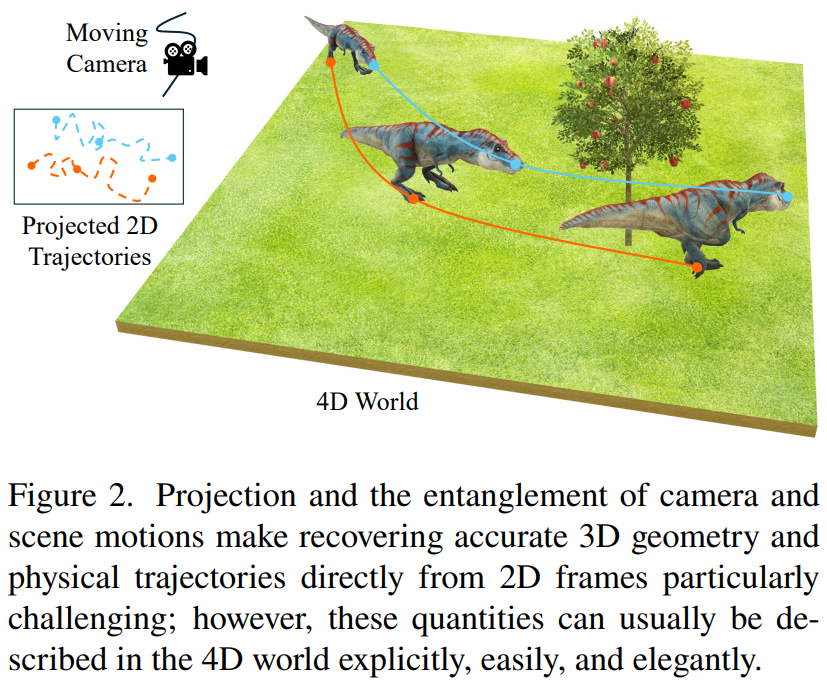
1. Existing video generation models do not have an explicit 3D spatial representation, so when the camera viewpoint changes or occlusion occurs as one object moves behind another, object shapes can become distorted and the sense of 3D structure can break down. In addition, video generation models cannot perfectly preserve the pixels from previous frames. Gaussians placed in 3D space, however, persist within a 3D representation, so with proper optimization they can maintain consistent geometry across multiple camera viewpoints (this gives some intuition for why many novel-view synthesis video generation papers use point clouds or 3DGS).
2. When motion is tracked on a 2D image, trajectories can become very complex because of perspective and camera shake, whereas in the original 4D (3D) coordinates, motion is much simpler and more regular because it follows physical laws. C4DD can also represent this motion as a continuous process, making it possible to naturally fill in arbitrary timestamps.
3. In a 2D video, changes caused by camera motion and object motion are entangled rather than separated, so there is no stable reference coordinate system. This makes learning difficult. In SeeU, however, depth estimation and tracking are used to separate the background and foreground, while the camera pose is explicitly disentangled from scene motion.

These considerations explain why SeeU is designed with the pipeline shown above.

Experiments

Datasets & Training details

The authors evaluate the method on 45 dynamic scenes collected from their own recordings and publicly available sources:

1. TAP-vid, a video point tracking benchmark
2. I2-2000FPS, a high-frame-rate dataset
3. AgiBot World, a robotics video set
4. Animal Kingdom dataset

These publicly available datasets are used as data sources.

They use a single NVIDIA A100 (80GB) GPU and optimize the model using the Adam optimizer. For the remaining training details of the 1st stage, 2nd stage, and 3rd stage, I recommend checking the paper directly.

Results

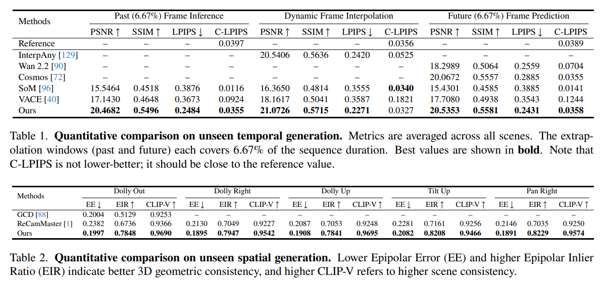
To evaluate Temporally Unseen Generation, as shown in Table 1, the authors infer past frames, Dynamic Frame Interpolation (between frames), and future frames, and evaluate them using PSNR, SSIM, LPIPS, and C-LPIPS. Because there is no single model that jointly performs inference for past, dynamic, and future frames, InterpAny, Wan2.2, and Cosmos, which perform dynamic or future inference, are used as existing SOTA baselines.

SoM and VACE are also methods from prior work, but they are extended so that they can handle past frames, frame interpolation, and future frames. VACE is extended to reconstruct the entire temporal range by masking the unseen frames, while SoM is somewhat forcefully extended to cover the entire temporal range by combining linear interpolation and linear extrapolation for motion estimation.

SeeU demonstrates substantially stronger continuous-time dynamics awareness and 3D geometric reasoning capability.

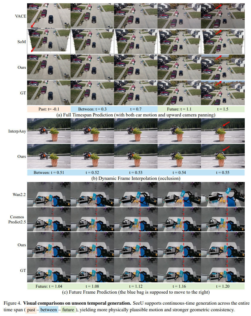
Figure 4 also shows that SeeU demonstrates substantially stronger continuous-time dynamics awareness and 3D geometric reasoning capability.

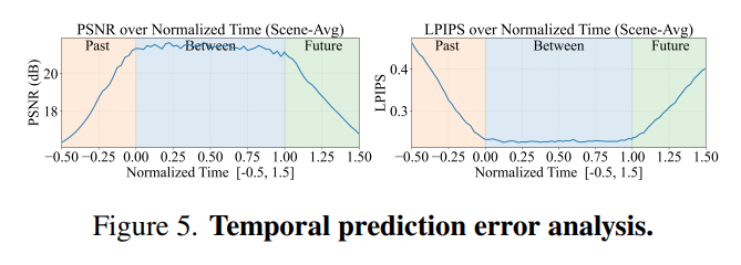
In addition, Figure 5 provides another interesting insight: in the extrapolated regions corresponding to the past 50% and future 50%, accuracy decreases approximately linearly as the temporal distance increases.

To evaluate Spatially Unseen Generation, as shown in Table 2, the authors compare multiple camera-control settings against GCD and ReCamMaster, which are video models that support camera control.

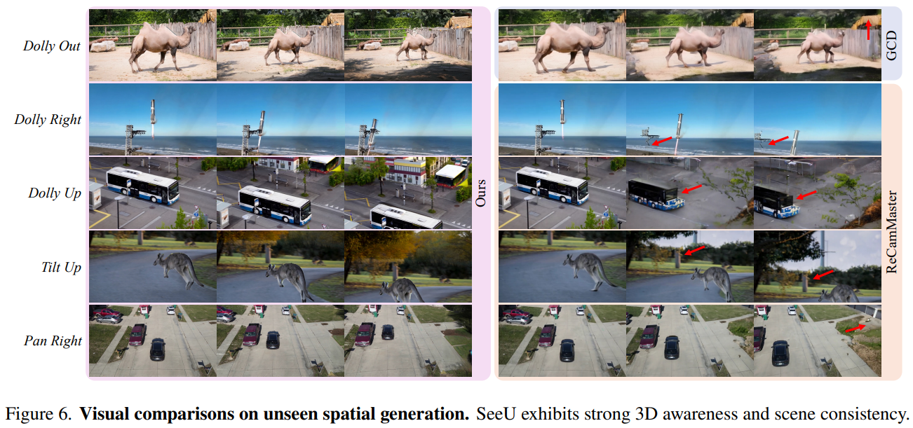
Table 2 shows that SeeU achieves higher geometric accuracy (EE and EIR) and scene consistency (CLIP-V) than all baselines, while Figure 6 shows that SeeU can render richer scene details.

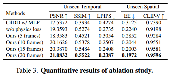
As shown in Table 3, the ablation study is conducted in three directions:

1. replacing the B-spline parameterization with plain MLP layers
2. setting the physics loss weight \(\lambda_{phys}\) to 0 to remove the effect of the physics loss term
3. varying the number of sparse input frames among 5, 10, 15, and 20

As shown in Table 3, the inductive bias of the B-spline for continuous dynamics appears to provide advantages in terms of smoothness and physical consistency. The physics loss term also seems to help stabilize continuous dynamics, and the method maintains robust performance even as the number of input frames becomes increasingly sparse (in my view as the reviewer of this paper, the input conditions of the models in Table 1 should be compared to determine more precisely whether there is truly an advantage with respect to the number of frames).

Contributions

1. The paper proposes a new concept, ‘SeeU,’ that directly learns continuous 4D dynamics from 2D projection images to generate unseen spatio-temporal regions (past/future/novel viewpoints) and enable sophisticated video editing.
2. It establishes, to the authors’ knowledge, the first ‘2D \(\rightarrow\) 4D \(\rightarrow\) 2D’ learning-framework paradigm in the literature, explicitly learning 4D physical dynamics from 2D input data and then re-projecting them into high-quality 2D video content.

Limitations & Future works

The input data used in this paper mainly consist of cases where foreground motion and changes in camera pose are smooth and clearly observable. In other words, the foreground does not change rapidly or irregularly from moment to moment, as in the case of basketball players, and the camera viewpoint does not change dramatically. Therefore, I expect the method may encounter difficulties in fully out-of-distribution scenarios.