[Paper Review, EN] WonderPlay: Dynamic 3D Scene Generation from a Single Image and Actions

Paper Information
Title: WonderPlay: Dynamic 3D Scene Generation from a Single Image and Actions
Authors: Zizhang Li, Hong-Xing Yu, Wei Liu, Yin Yang, Charles Herrmann, Gordon Wetzstein, Jiajun Wu
Venue: ICCV 2025 (Highlight)
Link: [Paper], [Project], [GitHub]

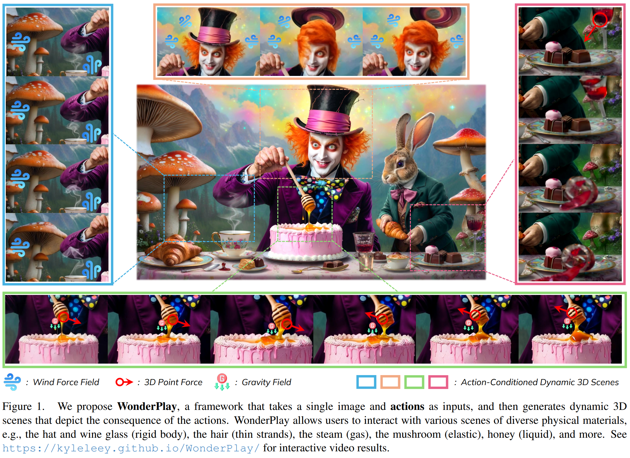
Teaser Image

Introduction

It is probably best to set one premise before reading.
Keep this sentence in mind: “WonderPlay is composed of a physics solver (essentially a physics engine) and a video diffusion model.”
(Note that this review does not cover how the physics solver works or its internal details.)

The paper lays out the limitations of a number of existing methods and techniques:

1. Existing methods for generating action-conditioned dynamic scenes cover only a limited range of dynamics, such as rigid and elastic bodies, and struggle to express general motion.
2. Existing video generation methods only produce 2D video and cannot generate a dynamic 3D scene; on top of that, the user has to know the resulting dynamic trajectory in advance and feed it in before a matching video can be generated. It is also an open question how such a dynamic trajectory should even be represented.
3. Existing world models remain at the level of camera control or text-based conditioning, so they cannot offer action-based interaction that responds to physical forces.
4. Existing methods for generating dynamic 3D scenes focus only on simple scenes and have no ability to physically simulate dynamics in response to a specific action input.

Having identified these limitations, the paper sets out to address them by using a physics solver and video diffusion together to build a “hybrid generative simulator”.

Method & Technical Details

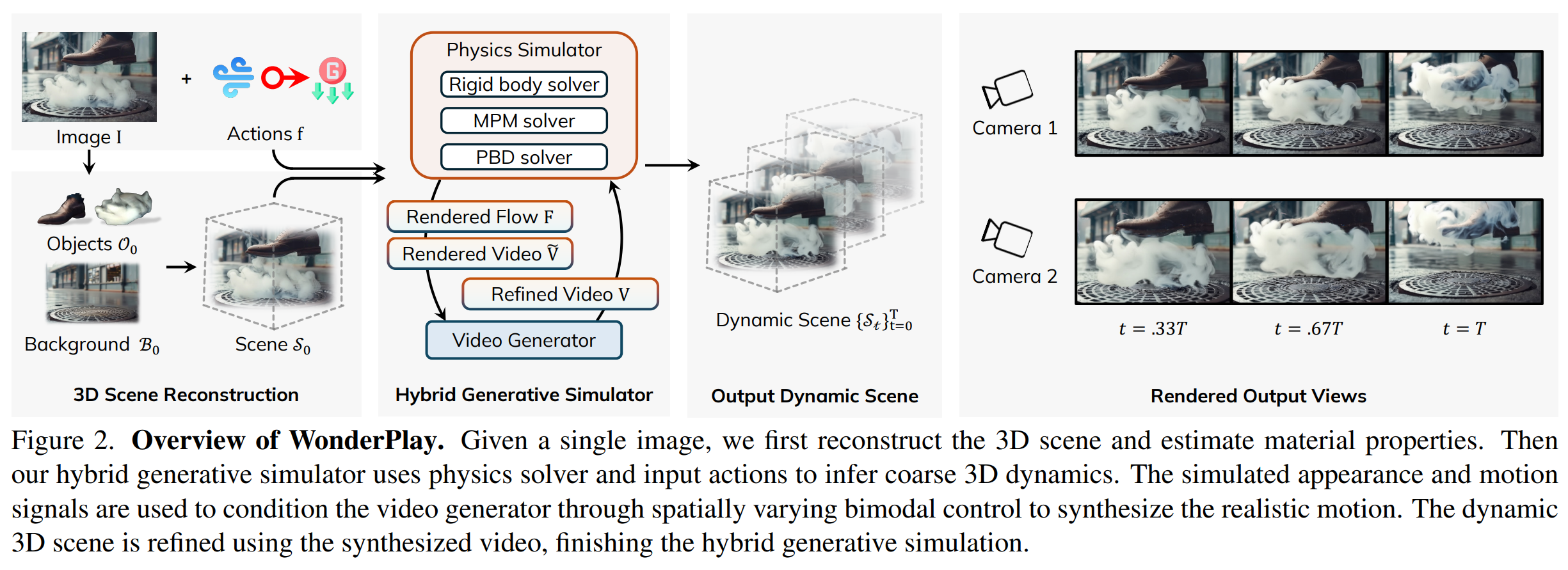
First, what is provided as input is a single image and actions. And the overall flow can be read as “physics solver -> video diffusion”.

Here the 3D scene is denoted $\mathcal{S}_t$, and this 3D scene consists of a background (\(\mathcal{B}_t\)) and objects (\(\mathcal{O}_t\)).
What we have to do is build the dynamic scene \(\{S_t\}_{t=1}^T\) from the input image $I$ and the actions $f_g$ (gravity), $f_w$ (wind), and $f_p$ (3D point force).

Background Reconstruction

The background is reconstructed and represented using the FLAGS (Fast Layered Gaussian Surfels) technique.
A detailed explanation of the algorithm will be given on the Preliminaries page. In short, the input image is split into several layers and unprojected into 3D space through depth estimation (e.g. monocular depth estimation, etc.). After that, the surfel parameters are optimized through an optimization step — that whole process is the technique called FLAGS.

So what exactly is a surfel?
-> Surfel is short for Surface Element, the basic unit used to represent the surface of an object in 3D space.
-> In this paper it is called a Gaussian surfel, and it carries (position, orientation, scale, opacity, color) information.

So there are $N_B$ Gaussian surfels (referred to simply as Gaussians from here on) making up the background, and you can think of them as being described by the Gaussian parameter set below.

\[\mathcal{B}_t = \{p^B, q^B, s^B, o^B, c^B_t\}\]

The symbols inside the braces denote positions, quaternions (rotation), scales, opacities, and RGB colors respectively — think of each as a means of describing a Gaussian.

Objects Reconstruction

A physics solver cannot recognize Gaussians as such; it mostly operates on meshes. Object reconstruction therefore does not stop at plain Gaussians — a dedicated model is used to convert the object into a mesh before use. The procedure is as follows.

1. Segment the object region from the input image first.
2. Represent the object as a 3D mesh with a model called InstantMesh.
3. Bind a Gaussian surfel to each vertex of the mesh and add edge and velocity information, completing the preparation for the physics solver’s computation.

Once this process produces a simulation-ready state, the paper calls it a “topological Gaussian surfel”. Writing it as a parameter set, just as in the background reconstruction, gives the following.

\[\mathcal{O}_t = \{E, v_t,p^O_t,q^O_t,s^O_t,o^O_t,c^O_t\}\]

The only difference from the background parameter set is the addition of the edge ($E$) and velocity ($v_t$) parameters.

In addition, so that an object can account for the physical laws of various substances, a material property $m$ intrinsic to the substance is defined, and a VLM classifies (estimates) it into one of six material types (rigid, elastic, cloth, smoke, liquid, and granular).

We now have $\mathcal{B}_0 \cup \mathcal{O_0} = S_0$ and the estimated $m$ ready, which lets us move on to the next stage.

1st stage: Physics Solver

As mentioned earlier, the overall flow is to pass through the physics solver and then refine with video diffusion.

In the first stage, the physics solver is used to build a coarse dynamic scene (\(\{\tilde{S}_t\}_{t=1}^T\)).
The process of building the dynamic scene over the entire horizon $T$ therefore repeats the formula below.

\[v_{t+1} , p_{t+1}^O, q_{t+1}^O = solver(\tilde{S}_t, f_g, f_w(t), f_p(t))\]

Two things can be read off this formula. First, the background Gaussians are not processed by the physics solver (i.e. they are static). Second, the current scene \(\tilde{S}_t\) is fed in so as to estimate the velocity, position, and quaternion at the next time step in order to obtain the scene \(\tilde{S}_{t+1}\) at \(t+1\). With that, the formula for the next time step’s scene makes sense.

\[\tilde{S}_{t+1} = \mathcal{B}_0 \cup \{ E, v_{t+1}, p_{t+1}^O, q_{t+1}^O, s_{0}^O, o_{0}^O, c_{0}^O\}\]

As the formula shows, the scene \(\tilde{S}_{t+1}\) at time $t+1$ is obtained from the background Gaussians together with the information estimated for the next time step. Notice, though, that the scale, opacity, and color parameters do not change and simply reuse their initial (\(t=0\)) values — from which we can infer the authors’ intent.

1. Either these are parts the physics solver estimates poorly or cannot estimate at all,
2. or they relate to visual quality rather than dynamics and will be handled later by the video diffusion anyway,
3. or it is simply to speed up inference.

2nd stage: Video Generator

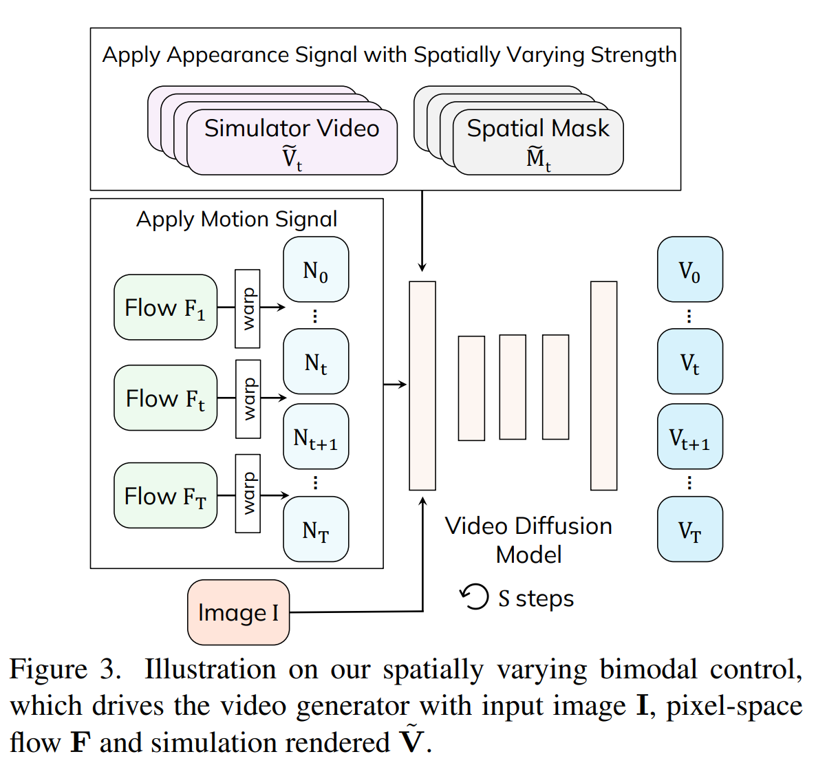
In the second stage, refinement is carried out on the basis of two concepts: motion control and RGB control

Motion control is the step that prepares the noise to be used by the video diffusion.

• First, the 3D velocity information \(\{ v_t \}_{t=1}^T\) of the Gaussian particles extracted by the physics solver in the 1st stage is projected onto a virtual camera view to render a 2D optical flow (\(F\)).
• After sampling a random Gaussian as the initial noise state $N_0$, the pixels are warped and aligned frame by frame along the flow vectors \(F\) obtained above, producing the warped noise \(N(F)\). The formula is as follows.

\[N_{t+1} = warp(N_t, F_{t+1})\]

• This guides the generation to follow the motion trajectory intended by the physics solver.

RGB Control

• First, the provisional 3D scenes \(\{ \tilde{S}_t \}_{t=1}^T\) obtained through the physics solver are rendered from the camera view to produce the RGB video \(\tilde{V}\).

\[V_{s_1} = \alpha_{s_1} \tilde{V} + \sqrt{1- \alpha_{s_1}^2} N(F)\]

• This formula carries out the forward process of the video diffusion. Building on the SDEdit technique, it tricks the timing at which denoising begins.
• Using this formula, restoration therefore starts not at the very first step of the diffusion model (\(S\), i.e. the maximum step) but at the intermediate step \(s_1\).

Spatially Varying

• There is an important point here. Hallucination in video diffusion is an unavoidable problem. To address it, the paper separates the background from the objects when denoising.
• The key concept is that the background does need refinement, yet in the output it should remain as static and unchanged as possible, whereas objects are exactly where active physical interaction has to take place. The paper therefore judges that the background needs fewer denoising steps and the objects need more steps than the background.
• If the \(s_1\) step from RGB control above is the number of steps the objects require, then the background needs only the smaller \(s_2(<s_1)\).

\[\hat{V}_{s_2} = M \odot V_{s_2} + (1-M) \odot (\alpha_{s_2}\tilde{V}+\sqrt{1-\alpha_{s_2}^2}N(F))\]

• So, as in the formula above, the background and the objects are separated in advance with a binary mask; refinement proceeds with both present up to step \(s_2\), at which point the background portion is boldly discarded, a fresh forward process produces a background-specific \(V_{s_2}\), and the background and object regions are merged again before denoising continues.

Expressing the 2nd stage as a single formula:

\[V = g(F, \tilde{V}, I)\]

That is, the resulting video is generated from the optical flow, the video rendered from the coarse scene, and the original input image.

3rd stage: Updating scene dynamics

Now the \(V\) completed in the 2nd stage is used to update the coarse dynamic scene \(\{\tilde{S}_t\}_{t=0}^T\). This is updated through the photometric L1 loss

\[\min\limits_{\{c_t^B,\mathcal{O}_t\}_{t=0}^T} ||V-\tilde{V}||_1\]

In other words, it computes the pixel-wise difference between \(V\), the high-quality video refined by the 2D diffusion, and \(\tilde{V}\), the output of the physics solver from the 1st stage. Backpropagating this loss updates the motion trajectories and velocity information of the Gaussians scattered in 3D space (\(O_t\)), as well as the color parameters of the background Gaussians (\(c_t^B\)) so as to reflect the real-time shading effects that arise during interaction.

For most AI papers, I personally recommend understanding the method first and looking at the overview figure only afterwards. The overview figure of this paper is as follows:

Experiments

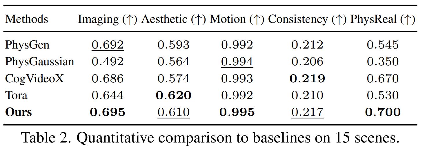
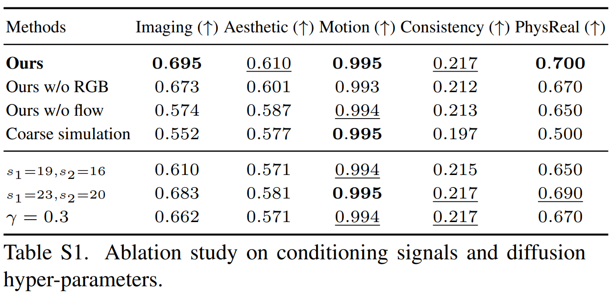
Quantitative evaluation was carried out over five metrics by applying VBench, a video quality assessment tool, against four baselines: the physics-based models PhysGen and PhysGaussian, and the conditional video generation models CogVideoX-I2V and Tora. The evaluation was run on a test set built from 15 demanding scenes (7 real photos and 8 carefully synthesized images) covering a range of materials such as cloth, rigid bodies, continua like sand, gas, and liquid. Among the five metrics, PhysReal was adopted as an evaluation protocol that leverages GPT-4o’s multimodal vision. A general explanation of the VBench evaluation protocol will additionally be uploaded to the Preliminaries page later.

Compared with the baseline models, WonderPlay recorded the best or second-best quantitative scores across the evaluation categories, including Aesthetic, Imaging, and PhysReal.

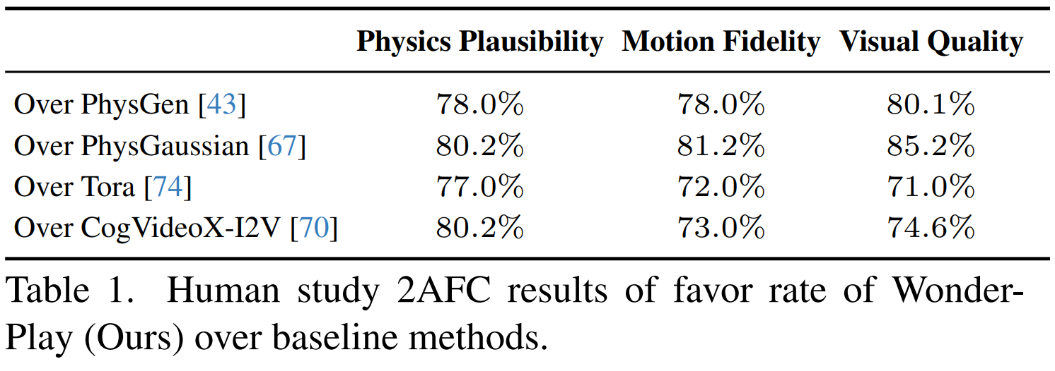
In addition, 200 users were recruited to perform a 2AFC evaluation. Across the three criteria — physics plausibility, motion fidelity, and visual quality — roughly 70–80% of evaluators, a clear majority, preferred WonderPlay’s output quality over the other models.

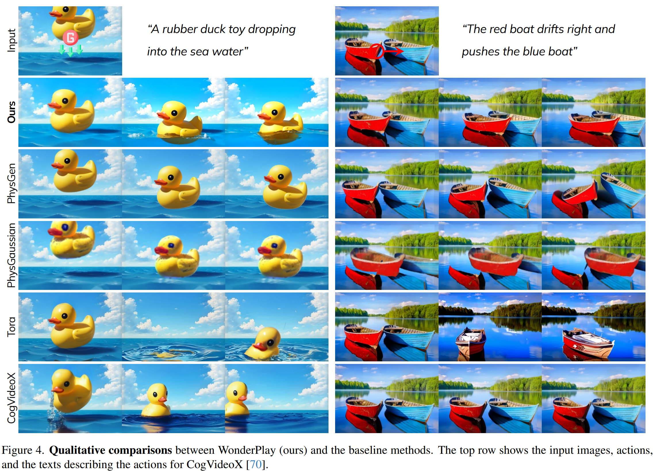
A qualitative evaluation was conducted against the four baseline models mentioned above.
In the duck-falling-into-water scene, Tora deformed the duck’s shape at random, while CogVideoX ignored the direction of the falling force and produced the contradiction of sliding the duck to the left out of nowhere. WonderPlay, by contrast, preserved both the way the duck descends below the water surface and its geometric shape intact thanks to the physics engine’s guidance, and by injecting video generation knowledge at the same time it even rendered the real splashing water waves and bubble details around the duck.

Now let’s look at how the shading effect was handled. In the scene where two boats collide and drift apart, PhysGaussian could not compute real-time shading because of the incomplete 3D Gaussian structure reconstructed from a single viewpoint, so the boat shapes reflected on the water stayed frozen and failed to follow the boats — the dynamic objects — in a natural way. With WonderPlay, the diffusion model updates the real-time shading effect and the realism of the reflections, expressing the phenomenon naturally.

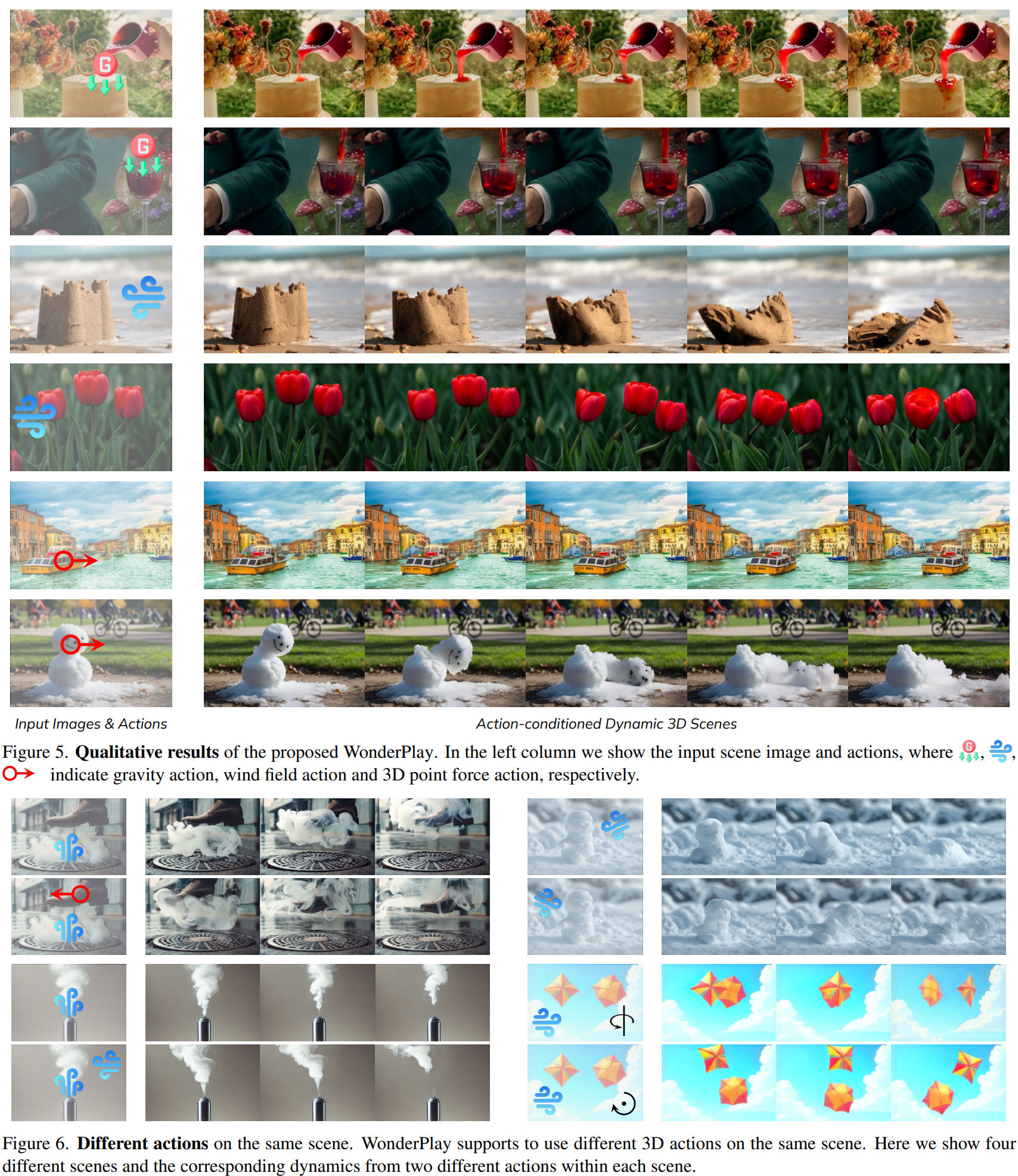
Experimenting with various other actions also shows that WonderPlay delivers solid performance.

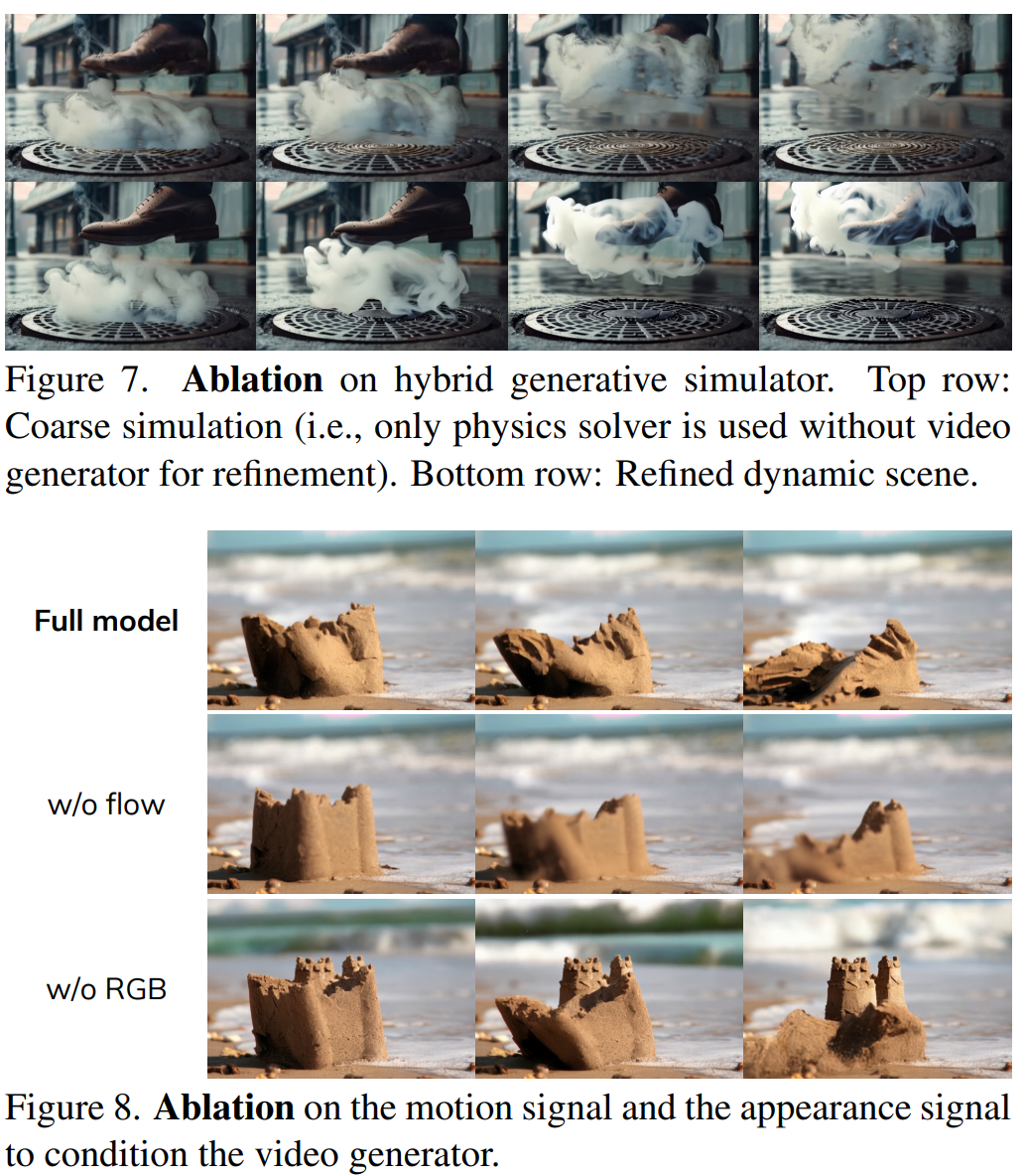
Beyond the quantitative evaluation, an ablation study lets us see how each module of WonderPlay affects the output.
Figure 7 shows the coarse version, where only the Gaussian physics solver is run without passing through the 2D diffusion, alongside the full model the paper advocates. In the smoke-emission scene, the coarse version failed to let the smoke unfurl smoothly because of the numerical viscosity problem inherent to every discrete-particle physics solver: the smoke clumped together stickily, like a sticky motion, and the particles swarmed very coarsely, like grainy artifacts. In the full model, however, the numerical viscosity noise is resolved and the geometric dynamics of real smoke swirling and dispersing through the air are restored in sync.

Experiments were also split into the case where the optical flow information — the pixel trajectories computed by the physics solver — is entirely excluded from the generator’s conditioning, i.e. the warped noise \(N(F)\) is not generated (w/o flow), and the case where the coarsely rendered \(\tilde{V}\) from the physics simulator is not injected as a condition into the generator (w/o RGB).

In the w/o flow case, the rough outward appearance (\(\tilde{V}\)) is preserved, but because there is no noise skeleton to guide the direction of pixel flow between frames, it fails to depict the fine rolling of sand grains or the detailed dynamic motion of smoke, and smearing occurs along the temporal axis. In the w/o RGB case, the generator’s degrees of freedom exceed their limit and hallucination becomes severe: an out-of-nowhere pile of sand castle spawns on its own and surges up behind the background, and the tile texture of the static background — which should stay still — keeps changing from moment to moment. An additional ablation study using VBench was also conducted, as shown below.

Contribution

Now let’s look at the paper’s contributions. They are most often written at the very bottom of the introduction, but it is good to go over the contribution items at the end as a way of wrapping up. The contributions this paper presents are as follows:

1. Solving a new problem that supports diverse physical materials: the paper sets out to solve the challenging problem of generating dynamic 3D scenes with diverse physical materials, conditioned only on a single image and the user’s action inputs.
2. Proposing a hybrid pipeline: it proposes a hybrid framework that integrates a physics solver and a video generator model, responding appropriately to the input actions while simultaneously achieving high visual fidelity.
3. Through qualitative and quantitative evaluation under a variety of interaction scenarios, it demonstrates that the method surpasses existing purely physics-based approaches and video generation models in terms of visual quality and physical plausibility.

Limitations & Future work

So what is worth investigating further, and what is still lacking?

To begin with, a follow-up model called ‘PerpetualWonder’ has already been released as a paper. Reading it will reveal the limitations WonderPlay has. A review of that paper will also be published on this blog.

The limitations and future work below are written based on both the view of the author of this review post and what is disclosed in the paper:

First, at a glance WonderPlay looks like a framework built to handle diverse materials, but it cannot handle every kind of material. The rigid body solver, MPM solver, and PBD solver do provide guidance for handling a wider range of materials than previous approaches, but if the video diffusion can identify the material type through a VLM in the first place, then having a video diffusion pretrained on a wealth of information handle it would ultimately be more beneficial (because short of simply adding solver after solver, you cannot represent every material that exists in the world).

Also, this is not a framework centered on real-time processing; it amounts to no more than an animator that plays back what appears after a click. In that sense, long-term user interaction may still be difficult. And the variety of interactions available to the user is small. Extending this to real-time user interaction therefore looks like the natural follow-up research.