[Paper Review, EN] SonoWorld: From One Image to a 3D Audio-Visual Scene

Paper Information
Title: SonoWorld: From One Image to a 3D Audio-Visual Scene
Authors: Derong Jin, Xiyi Chen, Ming C. Lin, Ruohan Gao
Venue: CVPR 2026
Link: [Paper], [Project], [GitHub]

Teaser Image

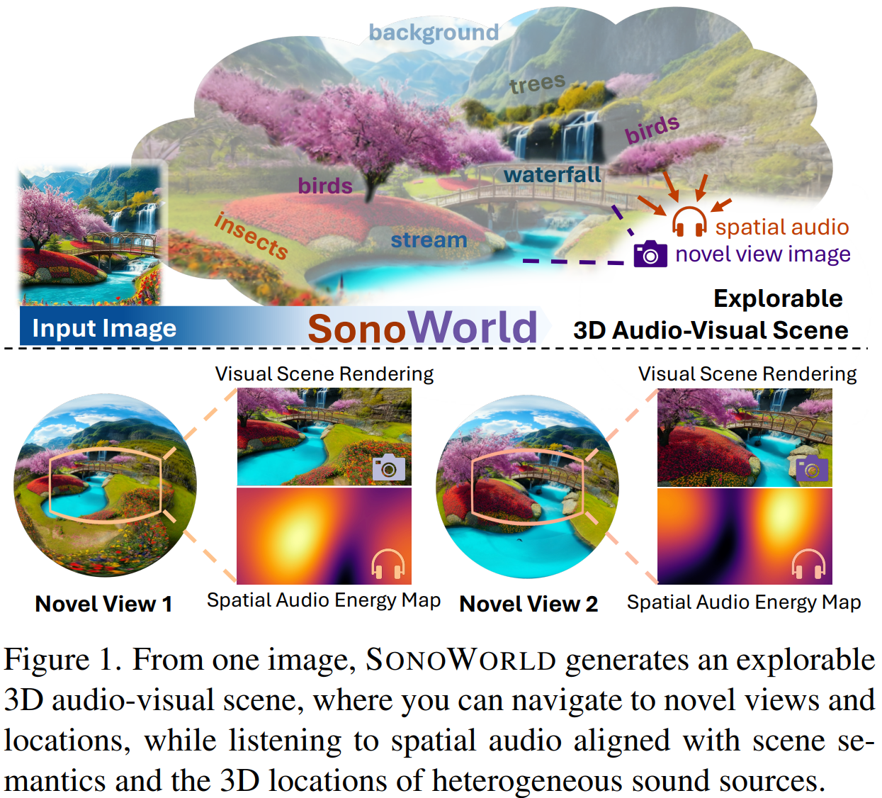
Introduction

Existing methods and techniques for creating immersive 3D scenes can generate photorealistic 3D worlds from a single image, but the authors argue that they remain perceptually incomplete without an auditory experience.

Therefore, the authors aim to build a training-free system that, from a single image, generates a coherent 3D scene together with a spatial sound field and supports user interaction.

To achieve this, there are three main challenges:

1. Scene-level audio generation must compose sound sources of diverse types and scales, including point sources, areal sources, and ambient soundscapes.
2. The system requires holistic semantic scene understanding to infer what is likely to make sound, how it should sound, and how loud it should be.
3. All generated sounds must be grounded at plausible 3D locations inferred from the image and rendered with perceptually realistic spatial effects.

Related research areas have the following limitations (you can skip this part if you are not interested in the research context.):

• This paper follows existing panoramic methods that outpaint a coherent 360-degree panorama and lift it into 3D through depth alignment and Gaussian optimization, but differs by jointly modeling spatial audio together with the visual scene.
• In prior spatial audio generation work, Sonic4D extends spatial audio generation to 4D dynamic scenes, but is limited to single objects, narrow views, and offline processing. SonoWorld goes beyond these limitations by supporting point, areal, and ambient sources as well as real-time exploration.
• SonoWorld also distinguishes itself from prior work on sound localization in visual scenes and Audio-Visual Source Separation. Rather than merely tracking where sound occurs in a visual scene or separating a mixed recording into individual audio components, it uses a VLM to discover potential sound sources in the generated 3D panoramic scene, ground them in 3D space, and directly generate new spatial audio for all sound sources located in the generated 3D visual scene.

The Image2AVScene Task

Ambisonics Concept

1. Spatial Sound representation

Ambisonics is a method for compactly representing “what sound is heard from which direction in the 360-degree space around me” using a small number of audio channels.

SonoWorld directly computes these Ambisonics channels using the locations of sound sources placed in the 3D scene.

Let us go through it step by step.

Ordinary mono audio that we typically hear (i.e., non-spatial audio) can be written as

\(a(t)\) which represents only how the sound changes over time.

For spatial audio, we also need to know the direction from which the sound arrives:

\[a(\theta, \phi, t)\]

where \(\theta=azimuth, left-right direction\) and \(\phi=elevation, up-down direction\) are used as parameters. It is easiest to understand this by imagining a sphere:

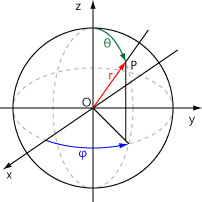
2. Spherical Harmonics

The problem is that directly storing sound for every direction over 360 degrees would require a large amount of storage and would also make real-time sound rendering difficult. Instead, Ambisonics represents the entire sound field using a small number of basic spatial patterns.

Let us denote each basic spatial pattern as:

\[Y_l^m(\theta, \phi)\]

When we input \(\theta, \phi\) for a specific direction, this function returns a weight for that direction. In other words, it is a pattern that assigns different weights to different directions over the sphere.

A full explanation would naturally lead into the Fourier Transform, but that would make this section too long. For now, it is enough to think of this as a “basis representing a particular 3D directional pattern”. Since basis is simply a standard term from linear algebra, I will not go deeper into it here.

In short,

Just as sin/cos act as basis functions in the Fourier Transform, spherical harmonics act as basis functions on the sphere.

3. Ambisonics coefficient

Equation (1) in the paper is

\[a(\theta, \phi, t) \approx \sum_{l=0}^L \sum_{m=-l}^l Y_l^m (\theta, \phi)a_{l,m}(t) = y_L(\theta, \phi)^T \mathcal{a}_L(t)\]

as shown above.

Here, \(Y_l^m (\theta, \phi)\) is a spatial directional pattern, and \(a_{l,m}(t)\) is the audio waveform corresponding to that pattern (encoded in Ambisonics).

In other words, Ambisonics does not directly store the entire 360-degree sound field,

\[a_{0,0}(t), a_{1,-1}(t), a_{1,0}(t), a_{1,1}(t) ...\]

but instead stores it as multiple audio channels such as these.

These are the Ambisonics coefficients, i.e., the Ambisonics channels, referred to in the paper.

A simple way to understand Equation (1) is

Directional Sound = Spatial Basis (Weights) X waveform stored in the Ambisonics Channels

That is the basic idea.

4. Ambisonics order and FOA

The Ambisonics order \(L\) determines the spatial resolution of the representation.

The paper mainly uses First-Order Ambisonics, FOA, where \(L=1\).

The number of Ambisonics channels is \((L+1)^2\), so FOA uses four audio channels (as Eq(1) shows, when L=1, \(\sum\) produces four terms in total).

So in this paper, you can think of \(a_1(t) \in \mathbb{R}^4\).

5. Encoding a Point source into Ambisonics

The most important equation in this paper is Equation (2), rather than Equation (1).

\[\mathcal{a}_L^{\text{single}} (t) = \sigma(d)a_{\text{src}}(t)y_L(u)\]

• $a_{\text{src}}(t)$ is the original sound waveform.
• $u$ is the direction from the listener toward the source.
• $\sigma(d)$ is the distance-dependent sound attenuation.

A simple way to understand it is as follows.

Ambisonics = Original Sound $\times$ Direction Information $\times$ Distance Effect

6. 3-DoF and 6-DoF

A conventional Ambisonics recording captures the sound field at a fixed location, so it supports

\[R \in SO(3)\]

which corresponds to 3-DoF rotation through yaw, pitch, and roll.

However, when the listener moves to another position, both the direction and distance to the source change.

SonoWorld knows the 3D source locations, so when the listener moves, it can recompute u and d at the new position and reapply Equation (2).

Therefore,

3 rotation DoF + 3 translation DoF = 6-DoF

This makes 6-DoF exploration possible.

7. A Potentially Confusing Point

Equation (2) encodes the original mono source waveform into multiple Ambisonics channel waveforms by incorporating the source direction and distance.

Equation (1) takes those Ambisonics channel waveforms and forms a weighted sum using the Spherical Harmonics values for a particular direction (θ,ϕ), yielding the directional waveform of a virtual microphone facing that direction.

For a virtual microphone facing direction $\mathbf{u}_{\mathrm{query}}$, the waveform is

\[a_{\mathbf{u}_{\mathrm{query}}}(t) = \mathbf{y}_L(\mathbf{u}_{\mathrm{query}})^T \mathbf{a}_L(t)\]

as shown above.

It becomes easier to understand if we substitute Equation (2) into Equation (1).

\[\mathbf{a}_L(t) = \sigma(d)\, a_{\mathrm{src}}(t)\, \mathbf{y}_L(\mathbf{u}_{\mathrm{src}})\]

Substituting this into Equation (1),

\[a_{\mathbf{u}_{\mathrm{query}}}(t) = \mathbf{y}_L(\mathbf{u}_{\mathrm{query}})^T \left[ \sigma(d)\, a_{\mathrm{src}}(t)\, \mathbf{y}_L(\mathbf{u}_{\mathrm{src}}) \right]\]

Since $\sigma(d)$ and $a_{\mathrm{src}}(t)$ are scalars, we can move them outside,

\[a_{\mathbf{u}_{\mathrm{query}}}(t) = \sigma(d)\, a_{\mathrm{src}}(t)\, \mathbf{y}_L(\mathbf{u}_{\mathrm{query}})^T \mathbf{y}_L(\mathbf{u}_{\mathrm{src}})\]

therefore

\[\boxed{ a_{\mathbf{u}_{\mathrm{query}}}(t) = \sigma(d)\, a_{\mathrm{src}}(t)\, \underbrace{ \mathbf{y}_L(\mathbf{u}_{\mathrm{query}})^T \mathbf{y}_L(\mathbf{u}_{\mathrm{src}}) }_{\text{directional matching term}} }\]

where,

\[\mathbf{y}_L(\mathbf{u}_{\mathrm{query}})^T \mathbf{y}_L(\mathbf{u}_{\mathrm{src}})\]

if this term is large, the direction faced by the virtual microphone and the actual source direction are well aligned in the Ambisonics basis, which can make the sound stronger in that queried direction.

Task Goal

\[\mathcal{G}: I \rightarrow \{V(p), A(p,t)\}\]

As shown in the equation, given a particular observer pose p, the goal is to construct the framework \(\mathcal{G}\) that produces the visual representation \(V(p)\) and \(A(p,t)\).

Here, \(V(p)\) is represented using 3D Gaussian splats, while \(A(p,t)\) is represented through point-cloud-based Ambisonics rendering:

\[a_L(t) = A(p,t) \in \mathbb{R}^{(L+1)^2}\]

Method & Technical Details

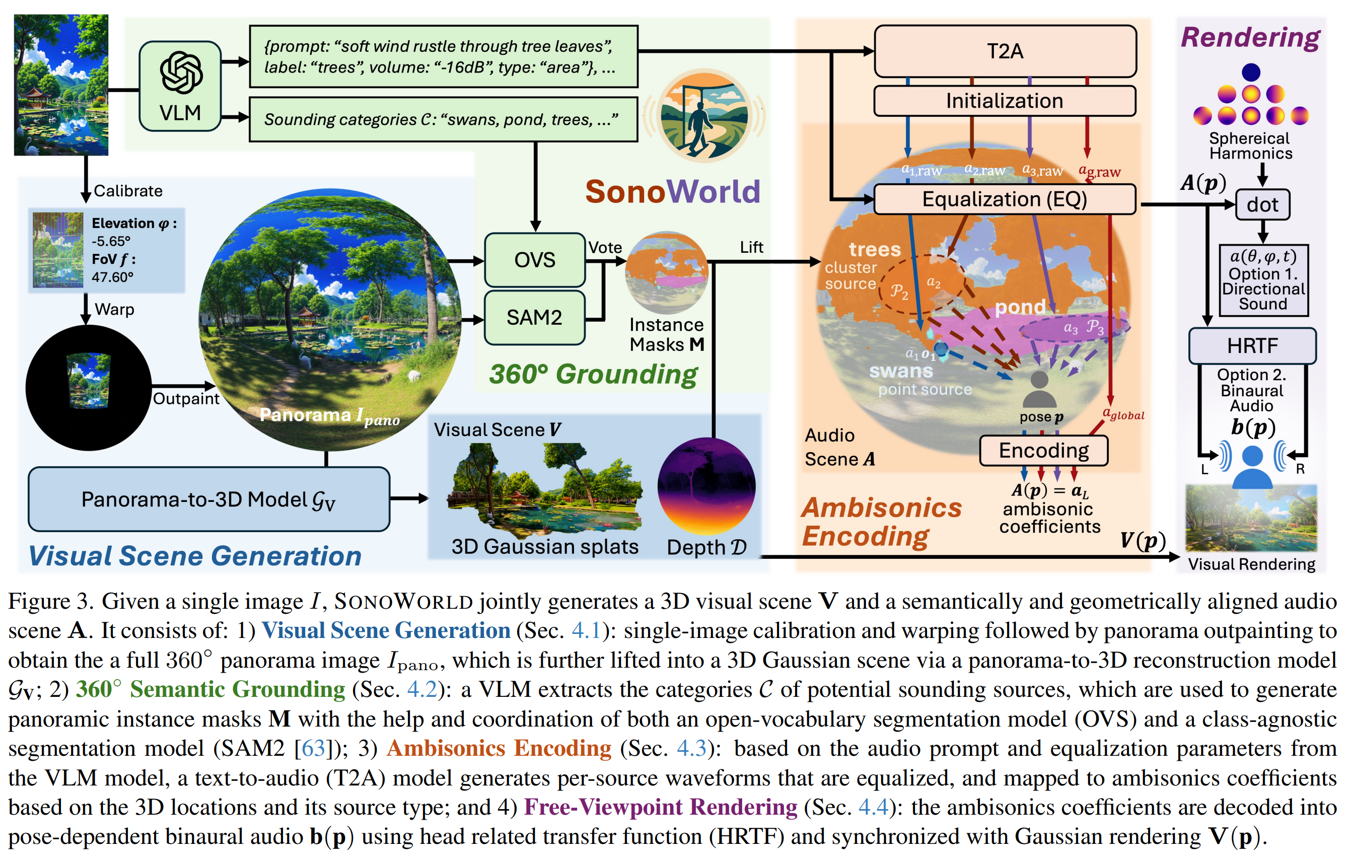
SonoWorld can be divided into four key techniques.

• First, generate a 360-degree panorama from a single input image and lift it into a 3D scene
• Second, identify potential sounding entities in the reconstructed 3D space and determine their locations
• Third, design an Ambisonics encoder that generates a spatial sound field
• Fourth, render immersive binaural audio from any listener pose

Panorama-Based Visual Scene Generation

Given a single image, many existing methods assume that the image is captured with a level camera looking straight ahead. However, this assumption can cause misalignment when the input image is tilted or captured at a different elevation. SonoWorld therefore begins by calibrating the input image.

\[(\phi,f) = Calib(I) ,\]

Using GeoCalib on the input image \(I\), the method estimates the gravity direction and camera FOV to obtain the camera elevation and FoV \((\phi, f)\). Next, to reproject the perspective image \(I\) into an equirectangular panorama, it uses a warping operator \(\mathcal{W}_G\) based on a Gaussian Pyramid. This operator performs multi-scale anti-aliased sampling, after which the warped image is passed to the WorldGen outpainting model \(g_{outpaint}\) to generate a 360-degree panorama:

\[I_{pano} = g_{outpaint}(\mathcal{W}_G(I, \phi, f))\]

The completed panorama is then lifted into a 3D scene using an existing panorama-to-3D reconstruction method:

\[V = \mathcal{G}_v(I_{pano})\]

For this step, the method uses either the Marble model or HunyuanWorld 1.0 to construct a photorealistic 3D environment.

360° Audio-Visual Semantic Grounding

This stage identifies which objects in the 3D scene are likely to produce sound and determines exactly where those objects are located in 3D space.

First, the input image \(I\) is given to a VLM, which returns four types of information.

• a set \(C\) of candidate sound source categories
• point/clustered/ambient sound type classification
• a text prompt for MMAudio to generate the waveform
• an Amplitude equalization parameter that determines how loud each sound source should be

Now, given the category set \(C\), we need to determine where those sound categories appear in the panorama. For this, the method uses X-Decoder, an open-vocabulary segmentation model.

Because X-Decoder is trained on ordinary perspective images, the panoramic image \(I_{pano}\) is split into multiple overlapping perspective FoV images. Conditioned on the category, X-Decoder then predicts the corresponding category segmentation mask for each tile image:

\[M_{OVS, c}\]

However, because X-Decoder processes the panorama as multiple tiles, masks can break at tile boundaries and may be unstable over large regions such as the sky or ground. Therefore, SAM2 is used to extract another set of masks that cleanly capture object regions directly on the panorama. This also complements the strengths and weaknesses of the two models: X-Decoder provides semantic labels for segmentation masks, whereas SAM2 does not.

In other words, SAM2 produces the class-agnostic segmentation mask

\[M_{pano}\]

as its output.

The X-Decoder results then cast confidence-weighted votes on the SAM2 regions.

If the overlap and semantic confidence are sufficiently high, the corresponding SAM2 mask is adopted as the mask for that category. This yields \(M_c\) for each category \(c\), and finally:

\[M=\cup_{c\in C}M_c\]

which gives the final mask set.

However, these are still only 2D locations, so they must be lifted into 3D space. Since we already have the 3D scene \(V\), we render a depth map \(D\) from that scene and use each sound source mask \(M_i\) together with depth \(D\) to perform

\[P_i = Lift(M_i, D)\]

this lifting operation. A single source is then represented as

\[P_i = \{p_1, p_2, ... , p_N\}\]

a set of 3D points.

The paper denotes the collection of all source point sets \(P_i\) as \(P\) and explains that it represents the 3D locations of sounding objects in the scene.

However, if we inspect the SonoWorld GitHub code, it uses SAM3 instead of X-Decoder and SAM2. With the earlier X-Decoder + SAM2 setup, the method likely relied on IoU-based processing to obtain refined masks, whereas SAM3 can provide both semantic labels and precise region masks. This appears to remove the need to run two separate models and apply an additional filtering algorithm. In other words, because SAM3 itself can discover and segment instances from text concepts, the previous combination of SAM2 and X-Decoder is no longer necessary.

Ambisonics Encoding

In this stage, the method generates the sounds that will populate the scene and mathematically assembles the final 3D spatial audio signal.

First, the text prompts proposed by the VLM from image analysis are passed to the audio generation model MMAudio, which generates a sound appropriate for each object (\(a_{i,raw}\)) and a global background sound (\(a_{global}\)). Rather than using the generated waveform volume directly, the sound energy (\(v_i\)) predicted by the VLM is converted from decibels into a physical signal scale using the equation below and multiplied into the waveform:

\[a_i(t) = 10^{v_i/20}a_{i,raw}(t)\]

This completes the volume balancing for each sound.

Earlier, we separated the global background sound from the individual object sounds. Keeping the global component separate, let the grounded sources be \(\mathcal{O}\), which is divided into \(\mathcal{O}_{point}\) and \(\mathcal{O}_{cluster}\).

Conceptually, a point source is spatially compact enough to be represented by a single position, whereas a clustered source is spatially extended and is better viewed as producing sound from multiple locations rather than from one point.

The listener pose is also important for providing a sound field. Ultimately, user tracking must be supported to provide immersive spatial audio. The listener position and viewing direction (pose) are represented as follows:

\[p = [R, t] \in SE(3)\]

Here, t is the listener’s 3D position and R is the listener’s rotation. This lets us describe how the sound changes when the listener turns their head or moves. In addition, an attenuation effect based on the distance (\(d\)) between the source and listener is required. It is expressed as follows:

\[\sigma(d) = \frac{e^{-\alpha d}}{d}\]

Placing d in the denominator produces distance attenuation, making the sound quieter as the source gets farther away, while \(e^{-\alpha d}\) in the numerator models air absorption, which introduces additional attenuation as sound travels through air over longer distances.

In other words, this function reduces the sound level as distance increases.

We can now see that Ambisonics is composed of three types of source-based spatial audio:

\[A = A_{point} + A_{cluster} + A_{global}\]

Open the sections below to see how the Ambisonics contribution of each source type is computed.

Point source

Here, a point source represents the 3D point cluster \(P_i\) of source \(i\) using a single centroid \(o_i\).

The relative position vector is then

\[d_i = t - o_i\]

Earlier, we defined the Ambisonics encoding equation as follows.

\[a_L(t) = \sigma(d)a_{\mathrm{src}}(t)y_L(u)\]

Applying the same structure to a point source gives

\[A_{\mathrm{point}} = \sum_{i \in \mathcal{O}_{\mathrm{point}}} a_{i,L} \sigma(\lVert d_i \rVert) y_L\left( R^T \frac{d_i}{\lVert d_i \rVert} \right)\]

which gives the point-source contribution.

Here, however, \(u \rightarrow R^T \frac{d_i}{\lVert d_i \rVert}\). Why does \(R^T\) appear?

The normalized vector \(\frac{d_i}{\lVert d_i \rVert}\) is the source direction in 3D world coordinates. However, we want to know where the source is relative to the direction the listener is currently facing, so the listener rotation \(R\) is used to transform the direction into the listener coordinate frame.

\[y_L\left( R^T \frac{d_i}{\lVert d_i \rVert} \right)\]

Therefore, this expression gives the Spherical Harmonics values for the direction of source \(i\) in the listener’s current coordinate frame.

Let us summarize this briefly.

Intuitively, this complicated notation can be written as

\[\boxed{ \text{Point Ambisonics} = \sum_i \text{source waveform} \times \text{distance attenuation} \times \text{source direction SH} }\]

which is the intuitive interpretation.

In other words,

\[a_L(t) = \sigma(d)a_{\mathrm{src}}(t)y_L(u)\]

Point Source Ambisonics is obtained by evaluating this equation for each source and summing all of the results.

Clustered sources

A spatially extended source such as a river or waterfall is difficult to represent with a single centroid, so all 3D points in \(P_i\) are used:

\[A_{\mathrm{cluster}} = \sum_{i \in \mathcal{O}_{\mathrm{cluster}}} \frac{a_i}{\lvert P_i \rvert} \sum_{o \in P_i} \sigma\left(\lVert d \rVert\right) y_L\left( R^T \frac{d}{\lVert d \rVert} \right)\]

The only difference from a point source is that one source now contains multiple 3D points. In other words, for each of the many point sources inside a clustered source, we compute

\[\sigma(\lVert d \rVert)y_L(\text{direction})\]

We then sum all of these terms and divide by \(\frac{1}{\left \vert P_i \right \vert}\) to take the average.

In simple terms, \(\text{Clustered source} = \text{Average of point sources}\).

The authors provide one additional insight.

When a clustered source is treated as multiple point sources as in the equation above, each point has a different direction and therefore a different \(y_L\) value. Because the \(l>0\) components of Spherical Harmonics can take positive or negative values depending on direction, contributions from different directions may partially cancel when summed.

Therefore, when an areal sound surrounds the listener, the \(l>0\) directional components tend to cancel one another, making the perceived directivity less sensitive to head rotation.

Global ambience

Finally, sounds such as wind or very distant traffic are not treated as being attached to a specific 3D object.

In other words, no directional information is assigned to the global ambience.

\[A_{global} = a_{global} \begin{bmatrix} 1 \\ 0 \\ 0 \\ \vdots \\ 0 \end{bmatrix}\]

This is represented by the equation above.

Only the first channel is used because it corresponds to the \(l=0\) omnidirectional component.

Free-Viewpoint Rendering

Once the previous stages are complete, we need to render both visuals and binaural audio from the generated visual scene and Ambisonics so that the user can see and hear the result.

Binaural audio refers to headphone audio represented as separate left-ear and right-ear signals.

After the previous stages, at listener pose \(p\) we have

\[a_L(t) = A(p,t)\]

the corresponding Ambisonics signal.

For FOA, L=1, so you can think of this as four waveforms:

\[a_1(t)= \begin{bmatrix} a_{0,0}(t) \\ a_{1,-1}(t) \\ a_{1,0}(t) \\ a_{1,1}(t) \end{bmatrix}\]

For the visual scene, the 3DGS renderer simply produces the camera image \(V(p)\) at pose \(p\).

How can Ambisonics be delivered as left/right-ear audio? HRTF provides the answer.

HRTF is a filter that describes how a sound arriving from a particular direction reaches the left and right ears after interacting with the listener’s head and ears.

For HRTF-based binaural rendering, the paper denotes the time-domain filters as

\[h_{l,m}^{left}, h_{l,m}^{right}\]

More precisely, these are called HRIRs. As the equation shows, each Ambisonics channel is convolved with the corresponding filter. This computes how that Ambisonics channel would actually be perceived at the left and right ears.

For example, the equation computes

\[h_{l,m}^{left} * a_{l,m} ,\; h_{l,m}^{right} * a_{l,m}\]

for the corresponding channel.

The final equation is therefore:

\[\begin{bmatrix} b_{\mathrm{left}} \\ b_{\mathrm{right}} \end{bmatrix} (t) = \sum_{\ell=0}^{L} \sum_{m=-\ell}^{\ell} \begin{bmatrix} h_{\ell,m}^{\mathrm{left}} * a_{\ell,m} \\ h_{\ell,m}^{\mathrm{right}} * a_{\ell,m} \end{bmatrix} (t)\]

In other words, the convolution outputs for all Ambisonics channels are summed for the left ear, and the same is done for the right ear, producing the final binaural audio delivered to the user.

Experiments

Because there is no existing dataset or benchmark that evaluates which sound should be heard from which direction when a listener is at a particular position in 3D space, the authors use their newly collected SONOSCENE360 dataset for quantitative evaluation. The dataset contains paired 360° video and FOA audio. For qualitative evaluation and the user study, they additionally use both internet photographs and diffusion-generated images.

The problem is that there is no existing method that performs the same IMAGE2AVSCENE task as SonoWorld. Therefore, the authors adopt related visual-conditioned spatial audio generation methods as baselines and adapt their inputs to the SonoWorld setting. The compared methods are MMAudio, SEE-2-SOUND, ViSAGe, and OmniAudio. Among them, only MMAudio is a monaural audio generator; the others are spatial audio generation methods.

Importantly, the visual scene is provided by SonoWorld. Although each model requires a different form of input, the evaluation measures how well each method generates spatial audio from renderings of the same visual scene. See the paper for details on how the input to each baseline is prepared.

Quantitative Results

SonoWorld provides two pipeline variants:

• Open-Source version: uses HunyuanWorld-1.0 as the 3D reconstruction model and LLaVA-Next-34B as the sound-source proposal model (VLM)
• Proprietary version: uses Marble as the 3D reconstruction model and GPT-5 as the sound-source proposal model (VLM)

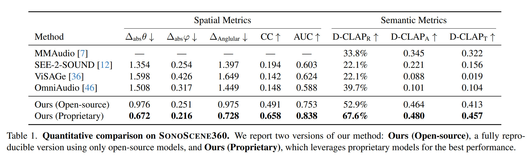
The table evaluates two groups of metrics: Spatial Metrics and Semantic Metrics.

In other words, it evaluates whether a sound is heard from the correct 3D direction and whether the appropriate type of sound is heard from that direction.

$\triangle_{abs \theta}$ denotes the azimuth error, $\triangle_{abs \phi}$ denotes the elevation error, and $\triangle_{Angular}$ denotes the overall 3D angular error. CC and AUC measure how similar the sound energy distribution over the sphere is to the GT when multiple sources are present.

As the table shows, the open-source version of the method already outperforms the previous methods overall. Replacing its components with proprietary models further improves performance.

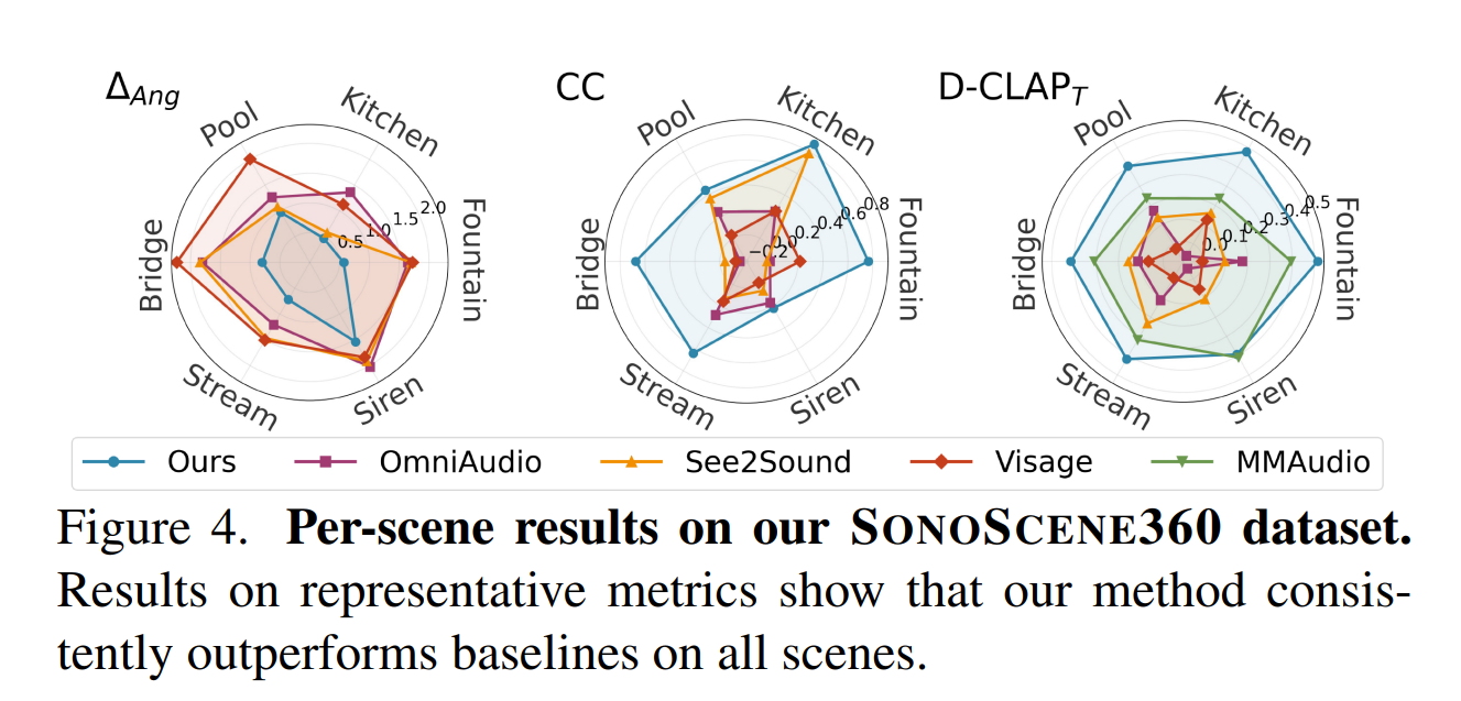
To show that the selected scenes are not biased in favor of SonoWorld, the authors also report metric results separately for each scene in SONOSCENE360. As the figure shows, they report consistently better performance than the baselines across all scenes.

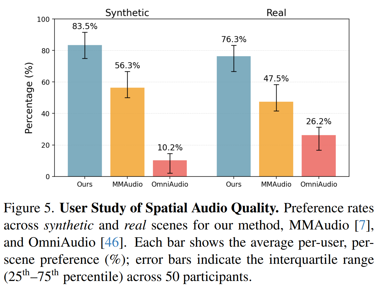
The authors also conduct a user study with 50 participants across 12 scenes. They perform three pair-wise comparisons:

• ours vs. MMAudio
• ours vs. OmniAudio
• OmniAudio vs. MMAudio

For each scene, the visual video is exactly the same across all methods, and only the generated audio differs.

Participants choose which audio is better based on spatial coherence and audio-visual semantic alignment. SonoWorld achieves the highest human preference on both real and synthetic scenes.

Qualitative Results

The paper first verifies whether users can freely navigate the 3D audio-visual scenes generated by SonoWorld while receiving the output in real time.

The paper states:

“For the Fountain scene, the audio callback is under 1 ms on an Apple M3 Pro, while one 256-sample buffer at 48 kHz spans about 5.3 ms.”

The audio setting is 48 kHz. This means that one second of an audio waveform is represented by 48000 samples, so each sample corresponds to \(\frac{1}{48000} sec\), or about 0.0208 ms. Calling the CPU after every individual sample would be inefficient, so the audio system processes multiple samples together as a buffer. In SonoWorld, the buffer size stated in the paper is 256 samples.

Here, when playback of the current 256 samples ends and the listener position changes, the audio callback must complete the following computations for the next 256 samples within the 5.3 ms playback duration so that the listener can continue hearing the result in real time:

\[\boxed{ \begin{gathered} \text{Audio system:} \\ \text{"Need the next 256 samples."} \\ \downarrow \\ \text{SonoWorld audio callback} \\ \downarrow \\ \text{Check current listener pose} \\ \downarrow \\ \text{Compute distance/direction to sound sources} \\ \downarrow \\ \text{Compute Ambisonics} \\ \downarrow \\ \text{HRTF decoding} \\ \downarrow \\ \text{Generate 256 Left/Right samples} \end{gathered} }\]

This makes uninterrupted real-time spatial audio playback possible as the listener moves.

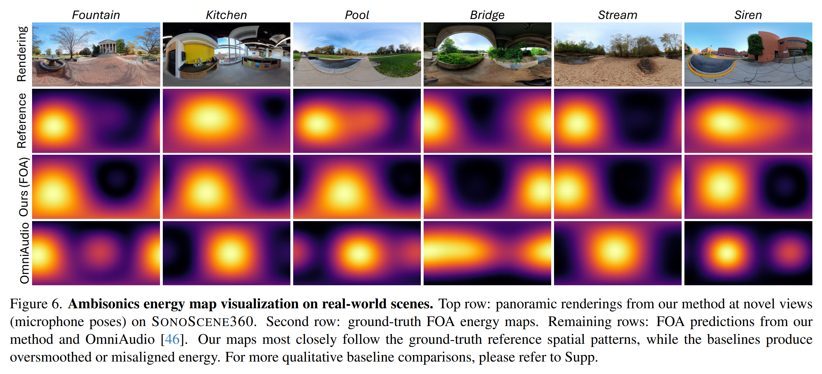
This figure shows the directions in 360° space where strong sound energy is present. It also shows that the directional distribution of the spatial audio is visually similar to the actual FOA.

Contribution

1. Defines “IMAGE2AVSCENE”, a new task that jointly generates an interactive 3D visual scene and spatial sound field, and introduces SONOWORLD, the first effective framework for the task
2. Collects and contributes SONOSCENE360, a dedicated evaluation dataset.
3. Substantially outperforms strong baselines across quantitative metrics, qualitative evaluation, and subjective perceptual evaluation, while also demonstrating applicability to several applications.

Limitations & Future work

One limitation is that the paper focuses on static 3D visual scenes; in other words, it does not handle 4D scenes with moving objects. Put simply, the work focuses on spatial audio rendering with user tracking. Extending the method to 4D scenes could require not only user tracking but also object tracking for moving sound sources, allowing source motion itself to affect the rendered spatial audio.